World ICT News

Responsive Web Design: A Deep Dive into CSS Media Queries

Jun 07, 2026

8 min read

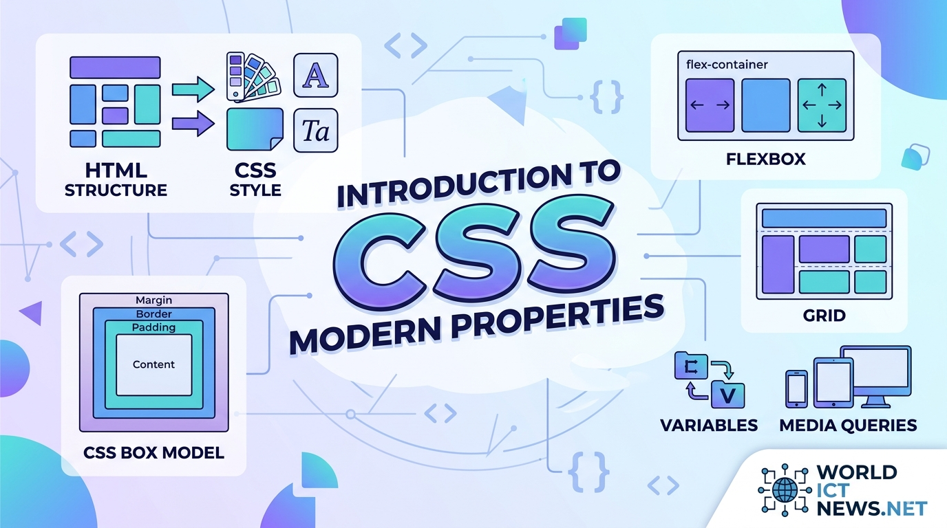
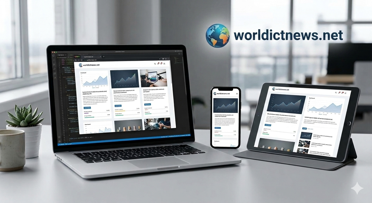
Responsive Web Design: A Deep Dive into CSS Media Queries

Mastering Responsive Web Design: A Deep Dive into CSS Media Queries. IntroductionThe modern web is accessed from an incredibly diverse ecosystem of hardware. A single website must render flawlessly on a 4-inch smartphone screen, an 11-inch tablet, a 15-inch laptop, and a 4K ultra-wide desktop monitor. In the early days of mobile internet, businesses built separate websites for mobile devices (often hosted on an m.dot subdomain like ://example.com). This approach doubled development time, fragmented search engine optimization (SEO) rankings, and created massive content management headaches.Responsive Web Design (RWD) solved this dilemma. Coined by Ethan Marcotte in 2010, responsive design is an approach where a website's layout dynamically adapts to the user's viewing environment based on screen size, orientation, and platform.At the heart of this design philosophy are CSS Media Queries. This comprehensive guide explores the core mechanics of creating fluid, responsive layouts using native CSS techniques, breakdown strategies, mobile-first workflows, and performance optimization rules.1. The Three Pillars of Responsive DesignBefore writing media queries, you must understand the three structural rules that make a layout responsive:+-------+| 1. THE VIEWPORT META TAG || Initializes layout scaling on mobile screens |+------+ | v+--------+| 2. FLUID GRID SYSTEMS || Elements scale fluidly using % / vw / vh / fr units |+--------+ | v+-------+| 3. MEDIA QUERIES || Applies structural design pivots at precise limits |+--------+The Mobile Viewport Meta TagBy default, mobile browsers try to emulate a desktop screen width (usually around 980 pixels) and scale the webpage down to fit the small screen. This results in microscopic text and unclickable links. To stop this emulation and tell the browser to render the page using the device's actual physical width, you must include this HTML tag inside your document's <head> region:html<meta name="viewport" content="width=device-width, initial-scale=1.0">Use code with caution.width=device-width: Sets the width of the page to match the screen width of the device.initial-scale=1.0: Sets the initial zoom level when the page first loads.Fluid Grids and Flexible ImagesA responsive layout avoids using fixed pixel layouts (e.g., width: 960px;). Instead, layout structural containers use relative units like percentages (%), viewport width (vw), viewport height (vh), or CSS Grid fraction units (fr).Similarly, images must be made flexible so they do not bleed outside their parent elements on smaller viewports:cssimg { max-width: 100%; height: auto;}Use code with caution.2. Anatomy of a Media QueryA media query consists of an optional media type and zero or more expressions that check for specific media features. If the conditions are true, the enclosed CSS rules are applied to the element.Syntax Breakdowncss@media media-type and (media-feature) { /* Targeted CSS Rules Go Here */}Use code with caution.@media: The CSS rule declaration that initializes the query block.Media Type: Specifies the category of the device. Common values include:screen: Used for computer screens, smartphones, and tablets (Most common).print: Used for preview screens and print layouts.all: Applies the styles to all media devices.Media Feature: The conditional expression checking the current state of the browser rendering layer. Common features include width, min-width, max-width, and orientation.3. Designing Breakpoints: Mobile-First vs. Desktop-FirstA breakpoint is the precise pixel threshold where a website's layout alters significantly via a media query to provide an optimized user experience. There are two opposite philosophical methodologies used to build responsive breakpoints.Methodology 1: Mobile-First (Highly Recommended)In a mobile-first workflow, you write your base CSS styles for the smallest screens first without any media queries. You then use progressive enhancement to add layout layers as the screen scales upward using min-width queries.This approach is highly performant because mobile devices do not have to parse complex desktop layouts, and it forces designers to prioritize essential content.css/* Base Styles: Applies to mobile viewports */.card-container { display: flex; flex-direction: column;}/* Tablet Layout Layer */@media screen and (min-width: 768px) { .card-container { flex-direction: row; flex-wrap: wrap; }}/* Desktop Layout Layer */@media screen and (min-width: 1024px) { .card-container { justify-content: space-between; }}Use code with caution.Methodology 2: Desktop-FirstIn a desktop-first workflow, the base styles define the full-scale desktop layout. You then use max-width media queries to subtract elements, shrink container grids, or stack navigation columns as the viewport scales downward.css/* Base Styles: Standard Desktop Layout */.sidebar { width: 300px; float: left;}/* Tablet / Mobile Adjustments */@media screen and (max-width: 767px) { .sidebar { width: 100%; float: none; }}Use code with caution.Standard Device Breakpoint FrameworksWhile you should ideally place breakpoints based on when your layout naturally breaks, using standard device ranges provides a highly reliable foundation:Screen RangeDevice CategoryCommon Breakpoint Target0px – 480pxSmartphones / Small MobileBase CSS Layer481px – 768pxTablets (Portrait) / Foldables@media (min-width: 481px)769px – 1024pxTablets (Landscape) / Netbooks@media (min-width: 769px)1025px – 1200pxStandard Laptops & Desktops@media (min-width: 1025px)1201px+Large Wide Desktops / 4K Monitors@media (min-width: 1201px)4. Practical Implementation: A Responsive 3-Card GridLet us construct a real-world example: a responsive product showcase grid that displays as a single stacked column on mobile, converts to a two-column grid on tablets, and scales into a clean three-column grid on desktop screens.HTML Structurehtml<!DOCTYPE html><html lang="en"><head> <meta charset="UTF-8"> <meta name="viewport" content="width=device-width, initial-scale=1.0"> <title>Responsive Grid Layout</title> <link rel="stylesheet" href="style.css"></head><body> <main class="grid-wrapper"> <article class="card"> <div class="card-image bg-blue"></div> <h2>Standard Analytics</h2> <p>Monitor your web data metrics in real-time with automatic cloud storage backups.</p> </article> <article class="card"> <div class="card-image bg-orange"></div> <h2>Secure Storage</h2> <p>Enterprise-grade threat protection layers safeguarding your customer profiles.</p> </article> <article class="card"> <div class="card-image bg-purple"></div> <h2>Automated Reports</h2> <p>Receive scheduled analytical summaries directly inside your team messaging apps.</p> </article> </main></body></html>Use code with caution.CSS Implementation (Mobile-First Workflow)css/* ======= 1. BASE STYLES: Mobile Viewports (0px - 480px) ====== */body { font-family: Arial, sans-serif; background-color: #f5f6fa; margin: 0; padding: 20px;}.grid-wrapper { display: grid; grid-template-columns: 1fr; /* Single column stack */ gap: 20px; max-width: 1200px; margin: 0 auto;}.card { background-color: #ffffff; border-radius: 8px; padding: 20px; box-shadow: 0 4px 6px rgba(0, 0, 0, 0.05);}.card-image { height: 150px; border-radius: 6px; margin-bottom: 15px;}.bg-blue { background-color: #3498db; }.bg-orange { background-color: #e67e22; }.bg-purple { background-color: #9b59b6; }/* ===== 2. TABLET UPGRADES: Viewports Larger Than 480px ===== */@media screen and (min-width: 481px) { body { padding: 40px; } .grid-wrapper { grid-template-columns: repeat(2, 1fr); /* Two-column grid setup */ }}/* ===== 3. DESKTOP UPGRADES: Viewports Larger Than 992px ===== */@media screen and (min-width: 992px) { .grid-wrapper { grid-template-columns: repeat(3, 1fr); /* Three-column grid setup */ } .card { transition: transform 0.3s ease; } .card:hover { transform: translateY(-5px); }}Use code with caution.5. Advanced Media Query CapabilitiesModern CSS provides capabilities beyond checking screen width. You can leverage advanced media features to create rich, context-aware web experiences.Checking Device OrientationYou can apply specific styles based on whether the user is holding their device in portrait or landscape mode:css@media screen and (orientation: landscape) { .hero-banner { height: 50vh; /* Reduces banner height to avoid pushing down content */ }}Use code with caution.Combining Multi-Condition ExpressionsYou can connect multiple logic rules within a single statement using operators like and, not, and commas (which act as an or operator).css/* Targets viewports strictly within tablet screen boundaries */@media screen and (min-width: 768px) and (max-width: 1024px) { .navigation-bar { background-color: #2c3e50; }}Use code with caution.Supporting Accessibility PreferencesModern operating systems allow users to flag accessibility preferences. Websites can read these parameters using media queries to provide a tailored browsing experience:css/* Detects if the user prefers dark mode layout schemes */@media (prefers-color-scheme: dark) { body { background-color: #121212; color: #ffffff; } .card { background-color: #1e1e1e; }}/* Disables animations for users who experience motion sickness */@media (prefers-reduced-motion: reduce) { * { animation: none !important; transition: none !important; }}Use code with caution.6. Performance Optimization and Best PracticesTo keep your responsive layouts smooth and organized, keep these industry best practices in mind:Avoid Over-nesting Media Queries: Keep media queries organized at the root level of your stylesheet, or append them cleanly beneath their corresponding element rules. Do not nest queries inside deep structural hierarchies.Use Relative Units (rem/em) for Breakpoints: Instead of hardcoding pixel breakpoints (768px), look into using relative root em units (48rem). Since 1rem is typically equal to 16px, relative units ensure your layout scales perfectly if a user changes their browser's default font size configuration.Minimize Reflow and Repaint Demands: Avoid altering layout properties (like width, margin, or float placements) inside high-frequency transition blocks. Changing structural dimensions forces the browser to recalculate the page layout, which can lead to layout jitter on lower-end mobile hardware.ConclusionResponsive web design is no longer an optional luxury—it is an essential requirement for the modern internet. By combining flexible grids with strategically configured CSS media queries, you ensure your applications provide a tailored user experience on any device.Adopting a mobile-first mindset ensures your code remains lightweight, organized, and optimized for performance. As you build your layouts, focus on cross-device compatibility, leverage modern flexbox or grid layouts, and use media queries to create seamless transitions between your layout variations.

Read Full Article

Digital Forensics in Autopsy Using Memory Artifacts

Jun 05, 2026

10 min read

Digital Forensics in Autopsy Using Memory Artifacts

Comprehensive Guide: Conducting Digital Forensics in Autopsy Using Memory Artifacts Extracted via Volatility 3 and Python. IntroductionWhen an enterprise endpoint is compromised, volatile memory (RAM) holds the most critical evidence of the intrusion. Threat actors increasingly deploy fileless malware, reflective DLL injections, and living-off-the-land binaries that exist purely within volatile storage loops, leaving no footprints on traditional disk drives.To analyze these complex attacks, forensic investigators use tools like Winpmem to extract raw memory dumps. However, a raw mem_capture.raw image cannot be directly ingested into structural database tools. Investigators must first bridge the gap between raw volatile dumps and structured timelines.This technical guide outlines the procedures for conducting a digital forensic investigation within Autopsy using structured data extracted from a Winpmem file. We will use Volatility 3 and custom Python automation scripts to automate artifact parsing, format raw outputs, and build a unified, time-correlated case file.1. Architectural Overview of the Forensic PipelineThe data analysis process follows a strict flow to preserve evidence integrity and ensure full forensic reproducibility:[Raw RAM (.raw)] ---> [Volatility 3 Engine] ---> [Python Extraction Script] | v[Unified Forensic Timeline] <--- [Autopsy Ingestion] <--- [Structured CSV Output]Acquisition Verification: Validate the raw RAM image file captured via Winpmem.Volatile Processing: Run Volatility 3 to extract raw text tables of processes, network sockets, and registry configurations.Python Automation: Execute a custom Python script to clean, parse, and reformat Volatility outputs into structured, Autopsy-compatible CSV datasets.Autopsy Integration: Ingest the structured files into Autopsy to build a comprehensive case timeline and correlate evidence.2. Setting Up the Automation EnvironmentTo follow this guide, ensure your forensic workstation has the following prerequisites configured:Volatility 3: Installed and accessible via your command-line interface (vol.py or volshell).Python 3.x: Installed with standard library access.Autopsy Forensic Browser: Installed (Version 4.19.3 or later recommended).Create a clean directory structure on your dedicated forensic workstation storage drive:bashmkdir -p /forensics/cases/incident_001/raw_datamkdir -p /forensics/cases/incident_001/vol_outputsmkdir -p /forensics/cases/incident_001/autopsy_csvUse code with caution.Place your raw memory capture (mem_capture.raw) into the /raw_data/ directory.3. Extracting Volatile Memory Layers via Volatility 3Before writing our automation script, we need to extract the raw artifact layers from the RAM dump. We will pull three critical data points: process structures, network connections, and the Windows system registry.Run the following commands in your terminal to generate the raw text data:bash# Extract active and hidden processespython3 vol.py -f /forensics/cases/incident_001/raw_data/mem_capture.raw windows.pslist > /forensics/cases/incident_001/vol_outputs/pslist.txt# Extract active network connections and listening portspython3 vol.py -f /forensics/cases/incident_001/raw_data/mem_capture.raw windows.netscan > /forensics/cases/incident_001/vol_outputs/netscan.txtUse code with caution.4. Automating Ingestion Setup via PythonVolatility 3 outputs data in human-readable text tables. To import this data into Autopsy as a logical data source, we need to reformat it into standard, comma-separated values (CSV) with explicit chronological headers.The following Python script automates this process. It reads the raw text outputs from Volatility, sanitizes white spaces, maps the columns, and writes clean CSV files that Autopsy can instantly index.The Parsing Script (vol_to_autopsy.py)Save the code block below as vol_to_autopsy.py on your workstation:python#!/usr/bin/env python3"""Forensic Automation Script: Volatility 3 Text Output to Autopsy-Compatible CSV Converter.Author: Digital Forensics Analyst"""import osimport reimport csvdef parse_pslist(input_path, output_path): """Parses windows.pslist output into a structured forensic CSV.""" if not os.path.exists(input_path): print(f"[-] Source file not found: {input_path}") return print(f"[+] Parsing Process List from: {input_path}") with open(input_path, 'r', encoding='utf-8') as infile, \ open(output_path, 'w', newline='', encoding='utf-8') as outfile: writer = csv.writer(outfile) # Write clean headers optimized for Autopsy logical file viewing writer.writerow(["PID", "PPID", "ImageFileName", "Offset", "Threads", "Handles", "SessionId", "Wow64", "CreateTime", "ExitTime"]) for line in infile: line = line.strip() # Skip Volatility header artifacts and system markers if not line or line.startswith("PID") or line.startswith("-") or line.startswith("Progress"): continue # Split lines by variable whitespace boundaries parts = re.split(r'\s{2,}', line) # Ensure the row matches expected Volatility column structures if len(parts) >= 8: pid = parts[0] ppid = parts[1] image_name = parts[2] offset = parts[3] threads = parts[4] handles = parts[5] session_id = parts[6] wow64 = parts[7] # Handle timestamps if process is active or terminated create_time = parts[8] if len(parts) > 8 else "N/A" exit_time = parts[9] if len(parts) > 9 else "Active" writer.writerow([pid, ppid, image_name, offset, threads, handles, session_id, wow64, create_time, exit_time])def parse_netscan(input_path, output_path): """Parses windows.netscan output into a structured forensic CSV.""" if not os.path.exists(input_path): print(f"[-] Source file not found: {input_path}") return print(f"[+] Parsing Network Scan Matrix from: {input_path}") with open(input_path, 'r', encoding='utf-8') as infile, \ open(output_path, 'w', newline='', encoding='utf-8') as outfile: writer = csv.writer(outfile) writer.writerow(["Offset", "Protocol", "LocalAddress", "LocalPort", "ForeignAddress", "ForeignPort", "State", "PID", "Owner", "CreatedTime"]) for line in infile: line = line.strip() if not line or line.startswith("Offset") or line.startswith("-") or line.startswith("Progress"): continue parts = re.split(r'\s+', line) if len(parts) >= 8: offset = parts[0] proto = parts[1] # Parse local and foreign socket points local_addr_port = parts[2].rsplit(':', 1) local_addr = local_addr_port[0] local_port = local_addr_port[1] if len(local_addr_port) > 1 else "N/A" foreign_addr_port = parts[3].rsplit(':', 1) foreign_addr = foreign_addr_port[0] foreign_port = foreign_addr_port[1] if len(foreign_addr_port) > 1 else "N/A" state = parts[4] pid = parts[5] owner = parts[6] # Reconstruct time blocks from ending segments created_time = " ".join(parts[7:]) if len(parts) > 7 else "N/A" writer.writerow([offset, proto, local_addr, local_port, foreign_addr, foreign_port, state, pid, owner, created_time])if __name__ == "__main__": # Define execution directories BASE_DIR = "/forensics/cases/incident_001" pslist_in = os.path.join(BASE_DIR, "vol_outputs/pslist.txt") pslist_out = os.path.join(BASE_DIR, "autopsy_csv/parsed_processes.csv") netscan_in = os.path.join(BASE_DIR, "vol_outputs/netscan.txt") netscan_out = os.path.join(BASE_DIR, "autopsy_csv/parsed_network.csv") # Run parsing scripts parse_pslist(pslist_in, pslist_out) parse_netscan(netscan_in, netscan_out) print("[+] Optimization Script Execution Completed Successfully.")Use code with caution.Running the ScriptExecute the parsing script from your terminal:bashchmod +x vol_to_autopsy.pypython3 vol_to_autopsy.pyUse code with caution.This generates clean CSV files in your /autopsy_csv/ folder, making the data ready for structured analysis.5. Step-by-Step Case Ingestion in AutopsyNow that your data is structured, you can import it into Autopsy to build your timeline and correlate evidence.Step 1: Initialize the Case RepositoryLaunch Autopsy.Click New Case from the welcome screen.Enter Case_Incident_001 as the Case Name.Set the Base Directory path to /forensics/cases/incident_001/ and click Next.Add your case number, investigator credentials, and initial summary notes. Click Finish to initialize the backend database.Step 2: Import the Extracted CSV Data SourcesRather than importing the large, unindexed raw file, we will add the structured memory datasets we created using our script.Select Data Source Type --> [Logical Files] --> Add Folder: `/forensics/cases/incident_001/autopsy_csv/`The Add Data Source wizard will automatically open. Select Logical Files as the data source type and click Next.Click Add and select the folder path containing your processed CSV files (/forensics/cases/incident_001/autopsy_csv/).Click Next to move to the Ingest Modules screen.Step 3: Configure Ingest Modules for Data ProcessingTo extract the most insight from your structured CSV files, enable these key ingest modules:Ingest ModuleAnalytical RoleFile Type IdentifierValidates the integrity of your CSV files and checks for spoofed extensions.Keyword SearchIndexes every text string, letting you search for specific IOCs (Indicators of Compromise), IPs, or malware names across all files.Interesting Files FinderFlags file alerts if specific conditions are met based on pre-defined rule sets.Click Finish to start the ingestion process.6. Forensic Artifact Correlation and Timeline AnalysisOnce Autopsy finishes processing the data, you can use its built-in analysis tools to connect the dots across your datasets.1. Analyzing the Unified TimelineClick the Timeline icon in the top toolbar to view a chronological visualization of your data.Filter your view around the exact time the security alert triggered. This lets you align the CreateTime of processes from parsed_processes.csv with network connection timestamps in parsed_network.csv. For example, you can see if a suspicious process like cmd.exe was spawned right as an inbound network connection was established on an unusual port.2. Hunting for Memory Threats with Keyword SearchesUse the Keyword Search field in the top-right corner to hunt for specific threats:Malicious IP Addresses: Search for external IP addresses flagged by your network monitoring logs. Autopsy will highlight every matching row within parsed_network.csv, instantly revealing the process ID (PID) responsible for the traffic.Process Masquerading: Search for common system binaries (e.g., svchost.exe, lsass.exe). Look for abnormal behaviors, such as multiple instances running from incorrect parent processes or mismatched non-system PIDs.7. Common Pitfalls and TroubleshootingAvoid these common mistakes to keep your analysis accurate and efficient:Mismatched Formatting Rules: Volatility plugins can occasionally change their text column layouts between software updates. If your Python script triggers an IndexError, open the raw text file in /vol_outputs/ and verify that the column layout matches the splitting rules in the regular expression parser.Corrupted Time Formatting: Autopsy reads timeline timestamps best when they are formatted in ISO 8601 (YYYY-MM-DD HH:MM:SS). If your Volatility output uses localized or truncated timestamps, adjust the string manipulation steps in your script to standardize the time fields before importing.Mixing Case Data: The "Logical Files" data source continues to reference your output folders actively. If you run multiple memory extractions within the same folder without updating your case files, you risk cross-contaminating your evidence. Always use unique case directories for each endpoint device you analyze.ConclusionBy combining Volatility 3, Python automation, and Autopsy, you create a highly efficient, repeatable digital forensics pipeline for memory analysis. Python handles the heavy lifting of parsing raw text into structured data, while Autopsy provides a powerful graphical suite for timeline correlation, keyword indexing, and evidence discovery.Using this structured workflow, incident response teams can quickly turn volatile RAM captures into actionable, timeline-driven forensic evidence, ensuring thorough documentation of sophisticated cyber attacks.

Read Full Article

A Complete Introduction to CSS Animation with Practical Examples

Jun 04, 2026

7 min read

A Complete Introduction to CSS Animation with Practical Examples

Mastering the Motion: A Complete Introduction to CSS Animation with Practical Examples. IntroductionIn the early days of web development, bringing movement to a webpage required heavy reliance on complex JavaScript libraries or resource-heavy Flash plugins. These methods frequently led to choppy performance, inflated file sizes, and poor mobile rendering. The introduction of CSS Animations fundamentally changed the web design landscape.CSS animations allow developers to transition elements from one configuration to another smoothly without touching a single line of JavaScript. By delegating animation rendering directly to the browser’s rendering engine—which can utilize hardware acceleration via the Graphical Processing Unit (GPU)—CSS animations deliver fluid, stutter-free performance.This comprehensive guide covers the core building blocks of CSS motion design. You will learn the mechanics behind the @keyframes rule, explore fundamental sub-properties, configure production-ready examples, and implement optimization strategies for modern websites.1. The Two Pillars of CSS AnimationEvery CSS animation relies on two interconnected components to function:The @keyframes Rule: The architectural blueprint of the animation. It defines the visual styles an element will hold at specific mathematical markers along a chronological timeline.The CSS Animation Properties: The engine configurations. Added directly to the target element's style block, these properties dictate how the blueprint executes (e.g., its speed, duration, repetition, and timing behavior).+--------------+| @keyframes Rule || (The Blueprint: 0% -> 50% -> 100%) |+---------------+ | v Applies to+---------------+| HTML DOM Element Class || (The Engine: Duration, Timing, Loops) |+--------------+2. Defining Keyframes: The BlueprintThe @keyframes rule establishes the states your element passes through during its animation sequence. You can specify these milestones using two distinct approaches.The Simple Approach: From/To SyntaxFor simple, two-state animations that move from a starting point to an ending point, use the from (0%) and to (100%) keywords.css@keyframes simpleFade { from { opacity: 0; } to { opacity: 1; }}Use code with caution.The Advanced Approach: Percentage SyntaxFor complex, multi-stage animations, use percentages. This allows you to break the timeline into precise increments, changing properties at various points along the way.css@keyframes multiStagePulse { 0% { transform: scale(1); background-color: #3498db; } 50% { transform: scale(1.15); background-color: #e74c3c; } 100% { transform: scale(1); background-color: #3498db; }}Use code with caution.3. Controlling the Engine: The 8 Sub-PropertiesTo run a @keyframes blueprint on an HTML element, you must configure its animation sub-properties. While short-hand methods exist, understanding the individual engine attributes is critical for fine-tuning motion.1. animation-nameLinks your target element directly to the unique identifier specified in your @keyframes rule.Example: animation-name: multiStagePulse;2. animation-durationSets how long the animation takes to complete one full cycle. It accepts values in seconds (s) or milliseconds (ms).Example: animation-duration: 3s; (Note: The default value is 0s, meaning no animation will occur unless this is explicitly set).3. animation-timing-functionControls the acceleration curve of the animation, dictating how it transitions through its keyframes.linear: Constant speed from start to finish.ease: Starts slow, accelerates quickly, then slows down at the end (Default value).ease-in: Starts slow, then accelerates steadily.ease-out: Starts fast, then decelerates smoothly.cubic-bezier(p1, p2, p3, p4): Allows you to author custom acceleration mathematical curves.4. animation-delaySpecifies a waiting period between the moment an element loads and the actual start of the animation sequence.Example: animation-delay: 500ms;5. animation-iteration-countDefines how many times the animation loop repeats. You can supply an exact integer or set it to run continuously.Example: animation-iteration-count: 3; or animation-iteration-count: infinite;6. animation-directionDetermines whether the animation plays forward, backward, or alternates between the two directions.normal: Plays forward from 0% to 100% (Default).reverse: Plays backward from 100% to 0%.alternate: Cycles forward, then backward on subsequent loops (0% $\rightarrow $ 100% $\rightarrow $ 0%).7. animation-fill-modeControls what styles are applied to the element before the animation begins (during a delay) or after it completes.none: No styles are applied outside the active timeline (Default).forwards: Retains the style properties of the final keyframe after the animation ends.backwards: Applies the styles of the first keyframe during an animation-delay period before execution.both: Applies both forward and backward rules simultaneously.8. animation-play-stateAllows you to pause and resume the animation dynamically, which is useful for user interactions like hover states.Options: running or paused.4. Practical Implementation: Code ExamplesLet’s apply these concepts to three distinct, production-ready design elements.Example 1: Creating a Loading Spinnerhtml<!DOCTYPE html><html lang="en"><head> <meta charset="UTF-8"> <title>CSS Loading Spinner</title> <style> body { display: flex; justify-content: center; align-items: center; height: 100vh; background-color: #f5f6fa; } /* The Spinner Container */ .spinner { width: 50px; height: 50px; border: 6px solid #dcdde1; border-top: 6px solid #2f3640; border-radius: 50%; /* Explicit Sub-Property Construction */ animation-name: spin; animation-duration: 1s; animation-timing-function: linear; animation-iteration-count: infinite; } /* Rotation Keyframe */ @keyframes spin { 0% { transform: rotate(0deg); } 100% { transform: rotate(360deg); } } </style></head><body> <div class="spinner"></div></body></html>Use code with caution.Example 2: Building an Attention-Grabbing Call-to-Action (CTA) ButtonThis example utilizes the shorthand animation property notation, combining name, duration, timing, and iteration rules into a single line.html<!DOCTYPE html><html lang="en"><head> <meta charset="UTF-8"> <title>Pulsing CTA Button</title> <style> body { display: flex; justify-content: center; align-items: center; height: 100vh; background-color: #1e272e; } .cta-button { padding: 15px 35px; font-size: 18px; font-family: sans-serif; font-weight: bold; color: #ffffff; background-color: #ffdd59; border: none; border-radius: 30px; cursor: pointer; box-shadow: 0 0 0 0 rgba(255, 221, 89, 0.7); /* Shorthand configuration: name | duration | timing | iteration */ animation: pulseGlow 2s ease-in-out infinite; } @keyframes pulseGlow { 0% { transform: scale(1); box-shadow: 0 0 0 0 rgba(255, 221, 89, 0.7); } 70% { transform: scale(1.05); box-shadow: 0 0 0 15px rgba(255, 221, 89, 0); } 100% { transform: scale(1); box-shadow: 0 0 0 0 rgba(255, 221, 89, 0); } } </style></head><body> <button class="cta-button">Join Now</button></body></html>Use code with caution.Example 3: Designing a Staggered Text Slide-In MenuBy using different animation-delay offsets on adjacent elements, you can create a sophisticated, staggered sequence where items slide in one after another.html<!DOCTYPE html><html lang="en"><head> <meta charset="UTF-8"> <title>Staggered List Animation</title> <style> body { display: flex; justify-content: center; align-items: center; height: 100vh; background-color: #2c3e50; font-family: Arial, sans-serif; } .menu-list { list-style: none; padding: 0; } .menu-item { background-color: #ecf0f1; margin: 10px 0; padding: 15px 40px; border-radius: 4px; font-size: 20px; color: #2c3e50; opacity: 0; /* Hidden initially before delay finishes */ /* Configuration using fill-mode to hold final state */ animation: slideIn 0.5s ease-out forwards; } /* Staggered Delay Intervals */ .menu-item:nth-child(1) { animation-delay: 0.2s; } .menu-item:nth-child(2) { animation-delay: 0.4s; } .menu-item:nth-child(3) { animation-delay: 0.6s; } @keyframes slideIn { 0% { opacity: 0; transform: translateX(-50px); } 100% { opacity: 1; transform: translateX(0); } } </style></head><body> <ul class="menu-list"> <li class="menu-item">Dashboard</li> <li class="menu-item">Analytics</li> <li class="menu-item">Settings</li> </ul></body></html>Use code with caution.5. Performance Optimization StrategiesWhile CSS animations are highly efficient, animating the wrong properties can cause performance drops, resulting in choppy frame rates on low-end mobile devices.The Browser Rendering PipelineWhen an element's style changes, the browser runs through three main rendering stages:Layout (Reflow): Calculates the size and position of elements on the page. Changing properties like width, height, top, left, or margin forces the browser to recalculate the layout for the entire document page structure. Avoid animating these properties.Paint: Fills in pixels, text colors, borders, and shadows. Properties like background-color, box-shadow, or color trigger paint operations.Composite: Organizes elements into distinct browser layers and draws them on screen.To achieve a buttery-smooth 60 Frames Per Second (FPS), limit your animations to properties handled entirely during the Composite stage:transform (Handles scaling, rotation, and translation calculations)opacity (Handles transparency values)Modern web browsers can offload these composite operations directly to the device's GPU, preserving main-thread processing power and ensuring highly fluid visual animations.ConclusionCSS animations provide a lightweight, high-performance toolkit for creating engaging user experiences. By mastering the relationship between @keyframes blueprints and your element properties, you can design everything from subtle UI micro-interactions to complex, staggered presentation layouts.As you design your animations, focus on hardware-accelerated properties like transform and opacity to keep your experiences fast, responsive, and cross-device compatible.

Read Full Article

Integrating Autopsy and Volatility for Advanced RAM Analysis

Jun 04, 2026

7 min read

Integrating Autopsy and Volatility for Advanced RAM Analysis

Digital Forensics: Integrating Autopsy and Volatility for Advanced RAM Analysis. IntroductionIn modern cybersecurity incident response, volatile memory (RAM) is a critical source of evidence. When a system is compromised, attackers often deploy sophisticated, fileless malware that resides exclusively in memory, leaving little to no trace on the physical hard drive. Traditional disk-based forensics can completely miss these active connections, injected code pieces, and hidden processes.To uncover these advanced threats, digital forensic investigators rely on specialized tools. This guide covers a powerful open-source forensic workflow: capturing physical memory using Winpmem, analyzing that memory image with the Volatility Framework, and integrating the results into Autopsy for comprehensive, timeline-based case investigation.1. The Critical Role of Volatile Memory ForensicsWhen an incident response team arrives at a compromised machine, they must prioritize data collection based on the Order of Volatility. Data in the CPU cache, routing tables, and RAM disappears the moment a machine is powered down or rebooted.Why RAM Analysis MattersActive Network Connections: Captures real-time sockets, listening ports, and remote IP addresses established by reverse shells or Command and Control (C2) servers.Decrypted Credentials: Reveals passwords, encryption keys, and session tokens stored in plaintext within memory buffers.Unpacked Malware: Code that is heavily obfuscated or encrypted on disk must unpack itself into RAM to execute, making it fully visible to memory analysis.Loaded Drivers and Modules: Pinpoints rootkits and malicious Dynamic Link Libraries (DLLs) injected into legitimate system infrastructure.2. Phase 1: Capturing RAM with WinpmemBefore you can analyze memory, you must capture it cleanly. Winpmem is a highly reliable, open-source memory acquisition tool for Windows environments. It uses a kernel-mode driver to map physical memory and write it out to a file (typically with a .raw, .dmp, or .img extension).Step-by-Step Acquisition ProcedurePrepare the Forensic Drive: Download the latest executable version of Winpmem. Always run Winpmem from an external, write-protected USB drive or a secure network share to avoid overwriting crucial evidence in the subject machine's RAM.Open an Elevated Terminal: Click the Start menu, search for cmd or PowerShell, right-click, and select Run as Administrator.Navigate to the Tool Location: Change directories to your external forensic drive:cmdcd D:\ForensicTools\ Use code with caution.Execute the Capture Command: Run Winpmem, specifying the output format and target destination. Use the standard raw output format for maximum compatibility:cmdwinpmem_3.3.rc3.exe --output C:\cases\mem_capture.raw --FORMAT rawUse code with caution.Note: Ensure the destination drive has enough free space to match or exceed the target machine's physical RAM capacity (e.g., a 16GB RAM system requires a minimum of 16GB of storage space).Calculate the Hash Value: Once the extraction finishes, immediately generate a cryptographic hash (SHA-256) of the generated image file to ensure chain of custody validation:cmdcertutil -hashfile C:\cases\mem_capture.raw SHA256Use code with caution.Record this hash in your forensic notebook.3. Phase 2: Processing the Memory Image with VolatilityOnce you have securely collected the .raw memory file, move it to your dedicated forensic workstation. Volatility is the industry standard framework for extracting structured information from raw memory dumps.While Volatility can isolate malware directly, processing raw memory listings in text form can make it difficult to visualize timelines. To solve this, we will configure Volatility to parse out core system files, which we will later import into Autopsy for deeper analysis.Essential Volatility Extraction CommandsDepending on whether you use Volatility 2 or Volatility 3, the syntax will vary slightly. Below are standard commands used to extract key forensic artifacts:Identifying Rogue ProcessesLook for suspicious parental architectures, unfamiliar process names, or hidden tasks:bash# Volatility 3python3 vol.py -f /cases/mem_capture.raw windows.pslistpython3 vol.py -f /cases/mem_capture.raw windows.pstreeUse code with caution.Spotting Active Network InfrastructureIdentify active or closed connections linking back to external malicious infrastructures:bash# Volatility 3python3 vol.py -f /cases/mem_capture.raw windows.netscanUse code with caution.Extracting Injected Code Blocks and DLLsUncover dynamic code blocks injected into legitimate background processes like svchost.exe or explorer.exe:bash# Volatility 3python3 vol.py -f /cases/mem_capture.raw windows.malfindUse code with caution.Exporting Registry Hives for Autopsy IntegrationTo build a cohesive timeline inside Autopsy, extract the primary Windows Registry hives hidden inside the RAM dump:bash# Create an output directory for the hivesmkdir /cases/extracted_hives# Dump the registry hives using Volatilitypython3 vol.py -f /cases/mem_capture.raw -o /cases/extracted_hives windows.registry.dumphivesUse code with caution.4. Phase 3: Integrating and Analyzing in AutopsyAutopsy is an intuitive, GUI-based digital forensics platform. While it is primarily used for hard drive images, its ingestion engine excels at compiling extracted registry structures, configuration files, and timelines into a centralized, searchable database.+---+ +--+ +--+| Winpmem (RAM) | ---> | Volatility Engine | ---> | Autopsy Workspace || .raw Memory Dump | | Artifact Extraction| | Comprehensive Case |+--+ +--+ +--+Step 1: Create a New Forensic CaseLaunch Autopsy.Click New Case.Enter a structured Case Name (e.g., Incident_Response_2026_001) and specify the base directory where case metadata will live. Click Next.Provide your investigator credentials, case number, and notes. Click Finish.Step 2: Add Extracted Memory Data SourcesInstead of importing the entire 16GB raw RAM file directly into Autopsy—which can slow down processing times—import the highly concentrated files, registry hives, and event logs extracted during Phase 2.Select Logical Files as the data source type, then click Next.Click Add and point the path explorer directly to your /cases/extracted_hives folder containing your Volatility output.Click Next to proceed to the Ingest Modules window.Step 3: Configure Ingest ModulesIngest modules are automated analysis tools that scan your imported files for evidence. For memory-extracted files, configure the following modules:[X] File Type Identifier (Detects spoofed file extensions)[X] Extension Mismatch Detector[X] Keyword Search (Input C2 IP addresses, suspicious domains, or known hacker aliases)[X] RegRipper (Automates parsing of the memory-extracted Registry hives)Click Finish to allow the background processing engine to start analyzing the data.5. Correlating the Evidence: Finding the Needle in the HaystackWith all your data organized inside Autopsy, you can now connect the dots across your various data sources to reconstruct the attack.1. Reconstructing the Attack TimelineClick the Timeline tool in the top Autopsy tool ribbon. This aggregates all data points into an interactive bar graph. You can filter the view to look at events that occurred around the exact minute the initial security alert triggered. This lets you see which registry keys were modified and which processes were spawned in memory right as the compromise happened.2. Finding Artifacts with RegRipperNavigate to the Results tree on the left sidebar and expand Extracted Data. Look for findings categorized by the RegRipper module:UserAssist Keys: Shows exactly which programs the attacker executed on the system, along with the precise execution timestamps.RunKeys: Uncovers any persistence mechanisms the malware added to the registry to ensure it restarts automatically if the computer reboots.3. Reviewing Keyword Search HitsIf your network monitoring tools flagged a suspicious destination IP address, look at the Keyword Hits folder in Autopsy. This shows you exactly where that IP address appears within the memory dump, whether it's embedded inside process strings, network buffers, or browser activity records.6. Common Pitfalls and Mitigation StrategiesSmearing the Memory Image: Running any tool on a live system alters its memory configuration slightly. Minimize this footprint by using lightweight command-line configurations for Winpmem and keeping all output paths pointed away from the local drive.Using Mismatched Profile Architectures: If you are using Volatility 2, selecting an incorrect operating system profile can lead to corrupted listings or failed parses. Always verify the target OS version using the windows.info module before running deep artifact extraction commands.High Memory Consumption During Analysis: Running Autopsy ingestion while simultaneously extracting artifacts with Volatility can easily overwhelm a standard forensic workstation. For stable performance, allocate a minimum of 32GB of RAM to your analysis workstation and assign specific CPU core limits within Autopsy's options menu.ConclusionCombining the strengths of Winpmem, Volatility, and Autopsy creates a comprehensive open-source workflow for volatile memory forensics. Winpmem safely captures evidence directly from RAM, Volatility decodes complex memory structures into accessible files, and Autopsy integrates everything into a searchable, timeline-driven case workspace.Using this structured approach, incident responders can thoroughly document threat actor activities, identify sophisticated fileless malware strains, and build resilient, audit-ready forensic cases.

Read Full Article

The Definitive Guide to T-Test Calculations Using PSPP

Jun 03, 2026

8 min read

The Definitive Guide to T-Test Calculations Using PSPP

The Definitive Guide to T-Test Calculations Using PSPP: Theory, Procedures, and Practical Examples. IntroductionIn quantitative research, comparing the mean scores of different groups or conditions is a fundamental task. Researchers often need to determine if an observed difference between two averages is statistically meaningful or simply a result of random sampling variation. To answer this question, analysts rely on the T-Test, a family of parametric statistical tests developed by William Sealy Gosset under the pseudonym "Student."While commercial statistical software suites like IBM SPSS are widely used for these calculations, their prohibitive licensing costs present significant barriers for independent researchers, students, and institutions in developing regions. PSPP serves as a powerful, free, open-source alternative. It mirrors the user interface, functionalities, and syntax language of SPSS, allowing users to execute complex statistical analyses seamlessly.This comprehensive guide provides step-by-step procedures for calculating the three primary types of T-Tests using PSPP: One-Sample T-Tests, Independent-Samples T-Tests, and Paired-Samples (Dependent) T-Tests. Each procedure is accompanied by a practical research scenario, a concrete example dataset, step-by-step data configuration instructions, and a framework for output interpretation.1. Fundamentals of the T-Test FamilyBefore executing commands in PSPP, it is vital to understand which T-Test fits your research design. All T-Tests compare means, but they differ based on where the data originates.The Three Varieties of T-TestsOne-Sample T-Test: Compares the mean of a single sample against a known or predetermined population mean or hypothetical test value.Independent-Samples T-Test: Compares the means of two distinct, unrelated groups (e.g., males vs. females, treatment group vs. control group) on the same continuous variable.Paired-Samples T-Test (Dependent T-Test): Compares the means of the same group of subjects at two different points in time or under two different conditions (e.g., pre-test vs. post-test scores).Core Statistical AssumptionsTo ensure the mathematical validity of your T-Test results in PSPP, your dataset should satisfy the following parameters:Continuous Scale: The dependent variable must be measured at the interval or ratio level.Independence of Observations: There must be no relationship between the observations within each group (crucial for Independent T-Tests).Normal Distribution: The dependent variable should be approximately normally distributed within each group.Homogeneity of Variance: For independent designs, the variances of the two groups should be roughly equal (tested via Levene's Test in PSPP).2. Procedure 1: One-Sample T-TestScenario & Example DatasetA university claims that its graduating seniors spend an average of 15 hours per week studying outside of class. A student researcher suspects the actual study time is different. They collect data from 8 randomly selected seniors.Hypothetical Population Mean (Test Value): 15Sample Data (Hours per week): 12, 14, 18, 11, 13, 16, 12, 10Data Entry in PSPPLaunch PSPP and select the Variable View tab at the bottom left.In row 1, type Study_Hours under the Name column. Set Decimals to 0 and type Weekly Study Hours under Label.Switch to the Data View tab.In the Study_Hours column, enter the 8 data points vertically into rows 1 through 8.Study_Hours ----------- 12 14 18 11 13 16 12 10 Execution StepsNavigate to the top menu bar and select Analyze $\rightarrow $ Compare Means $\rightarrow $ One Sample T Test...A dialog box will open. Select Weekly Study Hours [Study_Hours] from the left panel and click the arrow button ($\rightarrow $) to move it into the Test Variable(s) window.Locate the field labeled Test Value at the bottom of the box. Delete the default 0 and type 15.Click OK.Output InterpretationPSPP will display two tables in the Output Viewer: "One-Sample Statistics" and "One-Sample Test". One-Sample Statistics============Variable | N | Mean | Std. Deviation | SE. Mean----+-----+----+----+-----Weekly Study Hours | 8 | 13.25 | 2.60 | 0.92============= One-Sample Test==============Test Value = 15---------------- | | | | Mean | 95% Conf. Int.Variable | t | df | Sig. | Difference | Lower | Upper---+--+--+---+----+--+---Weekly Study Hours | -1.90| 7 | 0.100 | -1.75 | -3.92 | 0.42=============Mean: The sample mean is 13.25 hours, which is lower than the claimed 15 hours.t-value: The calculated test statistic is -1.90.df (Degrees of Freedom): Calculated as $N - 1 = 7$.Sig. (2-tailed): This is your p-value, which is 0.100.Statistical Decision: Because the p-value ($0.100$) is greater than the standard significance threshold ($\alpha = 0.05$), you fail to reject the null hypothesis. The difference between the sample mean (13.25) and the claimed mean (15) is not statistically significant.3. Procedure 2: Independent-Samples T-TestScenario & Example DatasetAn instructional designer wants to evaluate if a new interactive e-learning platform results in higher exam scores compared to traditional textbook learning. They test two independent groups of students.Group 1 (Textbook): 5 studentsGroup 2 (E-Learning): 5 studentsDependent Variable: Test Score (out of 100)Group 1 (Textbook) ScoreGroup 2 (E-Learning) Score75, 82, 78, 70, 8085, 89, 94, 80, 88Data Entry in PSPPUnlike spreadsheets where groups are placed side-by-side, statistical packages require a Grouping Variable (categorical code) and a Test Variable (continuous data).In Variable View, define two variables:Row 1: Name = Method, Type = Numeric, Decimals = 0, Label = Instructional Method.Row 2: Name = Score, Type = Numeric, Decimals = 0, Label = Exam Score.Click on the Value Labels cell for the Method variable. Define the groups:Value: 1 $\rightarrow $ Label: Textbook $\rightarrow $ Click Add.Value: 2 $\rightarrow $ Label: E-Learning $\rightarrow $ Click Add $\rightarrow $ Click OK.Switch to Data View and arrange the 10 cases vertically:Method | Score -------+------- 1 | 75 1 | 82 1 | 78 1 | 70 1 | 80 2 | 85 2 | 89 2 | 94 2 | 80 2 | 88 Execution StepsSelect Analyze $\rightarrow $ Compare Means $\rightarrow $ Independent-Samples T Test...Move Exam Score [Score] into the Test Variable(s) window.Move Instructional Method [Method] into the Grouping Variable box.Notice that the Define Groups button becomes clickable. Click it.Type 1 into Group 1 and 2 into Group 2. Click Continue.Click OK.Output InterpretationThe Output Viewer yields a group breakdown and a comprehensive split test matrix. Group Statistics=========Method | N | Mean | Std. Deviation | SE. Mean--+-+--+--+-----Textbook | 5 | 77.00 | 4.64 | 2.07E-Learning | 5 | 87.20 | 5.12 | 2.29========== Independent Samples Test=========Levene's Test for Equality of Variances: F = 0.081 | Sig. = 0.784------------- | t | df | Sig.(2-tail) | Mean Difference--+--+--+-+---Equal var. assumed | -3.31 | 8 | 0.011 | -10.20Equal var. not assumed| -3.31 | 7.92 | 0.011 | -10.20==========Step 1: Check Levene's Test. Look at Sig. = 0.784. Because this value is much greater than $0.05$, the variances are equal. We read the data from the row labeled Equal variances assumed.t-value and df: $t = -3.31$ with $8$ degrees of freedom.Sig. (2-tailed): The p-value is 0.011.Statistical Decision: Since $0.011 < 0.05$, the result is statistically significant. The E-Learning group achieved a significantly higher mean test score ($87.20$) compared to the Textbook group ($77.00$).4. Procedure 3: Paired-Samples T-TestScenario & Example DatasetA medical clinic evaluates a new 4-week exercise regimen designed to reduce systolic blood pressure. The researcher records the blood pressure of 6 participants before starting the program and immediately after completion.ParticipantPre-Test Score (mmHg)Post-Test Score (mmHg)114513821381323150142416015151351366142139Data Entry in PSPPBecause the samples are paired (dependent), each row must represent an individual subject with both measurements placed side-by-side.In Variable View, define two variables:Row 1: Name = Pre_BP, Label = Systolic BP BeforeRow 2: Name = Post_BP, Label = Systolic BP AfterSwitch to Data View and enter the data across 6 rows:Pre_BP | Post_BP -------+-------- 145 | 138 138 | 132 150 | 142 160 | 151 135 | 136 142 | 139 Execution StepsNavigate to Analyze $\rightarrow $ Compare Means $\rightarrow $ Paired-Samples T Test...Click on Systolic BP Before [Pre_BP] and then click on Systolic BP After [Post_BP].Click the arrow button ($\rightarrow $) to move the selected combination into the Paired Variables window as a linked pair (Pre_BP - Post_BP).Click OK.Output Interpretation Paired Samples Statistics=========Variable | N | Mean | Std. Deviation | SE. Mean---+-+--+--+---Systolic BP Before | 6 | 145.33 | 8.78 | 3.58Systolic BP After | 6 | 139.67 | 6.47 | 2.64========== Paired Samples Test========= | | | | Mean | 95% Conf. Int.Pair 1 | t | df | Sig.2 | Diff. | Lower | Upper-+-+-+-+--+--+--Pre_BP - Post_BP | 4.11 | 5 | 0.009 | 5.67 | 2.12 | 9.21==========Means Comparison: The mean blood pressure dropped from 145.33 mmHg before the program to 139.67 mmHg after.Mean Difference: The average net reduction per person was 5.67 mmHg.t-value and df: $t = 4.11$ with $5$ degrees of freedom.Sig. (2-tailed): The p-value is 0.009.Statistical Decision: Since $0.009 < 0.05$, the drop in blood pressure is statistically significant. The 4-week exercise program is an effective intervention for lowering systolic blood pressure.5. Alternative Execution: Using PSPP Syntax WorkspaceIf you want to bypass the graphical user interface or run your data analysis via scripting for reproducibility, you can use PSPP Syntax.Open a new window by choosing File $\rightarrow $ New $\rightarrow $ Syntax.Depending on your chosen analysis, paste one of the following code blocks:spss* --- COMMAND FOR ONE-SAMPLE T-TEST ---T-TEST /TESTVAL=15 /VARIABLES=Study_Hours.* --- COMMAND FOR INDEPENDENT-SAMPLE T-TEST ---T-TEST /GROUPS=Method(1, 2) /VARIABLES=Score.* --- COMMAND FOR PAIRED-SAMPLES T-TEST ---T-TEST /PAIRS=Pre_BP WITH Post_BP (PAIRED).Use code with caution.Highlight the desired block of text and select Run $\rightarrow $ Selection from the top menu.6. Troubleshooting Common PSPP ErrorsMissing Variables in the Selection Panels: If your variable does not appear in the T-Test selection list, check its Type in Variable View. String (text) variables cannot be used in mathematical mean comparisons. Change the type to Numeric.Incorrect Levene's Row Choice: For the Independent T-Test, if Levene’s test value Sig. is less than 0.05, you must reject the assumption of variance equality. In that case, read the metrics from the bottom row, labeled Equal variances not assumed (Welch's T-test adjustment).Empty Output Matrix: Ensure your variables do not contain non-numeric characters or unmapped values. PSPP will drop incomplete data points listwise, resulting in empty values if your datasets are small.ConclusionMastering the execution of T-Tests within PSPP allows you to make data-driven comparisons without relying on expensive software. Whether checking a single group against a standard benchmark, evaluating two distinct educational methods, or observing variations over time, following these structured procedures ensures accurate results and clear reporting for your research project.

Read Full Article

Calculating Descriptive Statistics for Grouped Data Using PSPP

Jun 03, 2026

7 min read

Calculating Descriptive Statistics for Grouped Data Using PSPP

Master Guide: Calculating Descriptive Statistics for Grouped Data Using PSPP. IntroductionIn data analysis, we often encounter datasets where individual raw scores are unavailable. Instead, the data is pre-arranged into intervals, ranges, or categories. This format is known as grouped data. Grouped data is highly efficient for summarizing massive datasets, tracking frequency distributions, and understanding demographic spreads. However, analyzing grouped data requires a fundamentally different statistical approach than analyzing unorganized raw data.To analyze this data without expensive software licenses, researchers turn to PSPP. PSPP is a powerful, open-source alternative to IBM SPSS. It replicates the SPSS user interface and syntax, making high-level statistical analysis accessible to everyone.This comprehensive article provides a step-by-step procedure for calculating descriptive statistics for grouped data using PSPP. You will learn how to structure your dataset, apply essential statistical adjustments, and interpret your output data effectively.1. Understanding Descriptive Statistics for Grouped DataWhen dealing with ungrouped data, computing the mean, median, or standard deviation is straightforward. You simply add up the scores or look for the exact middle value. With grouped data, individual identities are lost inside class intervals (e.g., ages 20–29, 30–39).To calculate statistics for grouped data, we must work with two primary components:Class Midpoints ($X_{m}$): The exact middle value of a class interval. This serves as the proxy value for all individual scores contained within that group.Frequencies ($f$): The number of observations or participants falling inside that specific interval.Statistical Adjustments in PSPPSoftware packages like PSPP are naturally built to calculate descriptive statistics from individual case rows. If you enter grouped data into PSPP normally, the software will read your frequencies as single, independent data points rather than group multipliers. To fix this, we must use a critical feature called Weight Cases. This instructs PSPP to treat your frequency column as a scale multiplier, ensuring your mean, variance, and standard deviation calculations are mathematically accurate for the total population size ($N = \sum f$).2. Preparing and Formatting Grouped Data for PSPPBefore launching PSPP, you must structure your grouped data correctly. Let us look at a practical sample scenario: analyzing the monthly operational costs of 50 small tech startups.Class Interval (Cost in USD)Frequency (Number of Startups)$1,000 – $2,0008$2,001 – $3,00015$3,001 – $4,00018$4,001 – $5,0009Step 1: Calculate the Class Midpoints ManuallyStandard statistical software cannot natively process a text range (like "$1,000 – $2,000") as a mathematical value. You must calculate the midpoint for each interval before data entry.$\text{Midpoint\ }(X_{m})=\frac{\text{Lower\ Limit}+\text{Upper\ Limit}}{2}$For Interval 1: $(1000 + 2000) / 2 = \mathbf{1500}$For Interval 2: $(2001 + 3000) / 2 = \mathbf{2500.5}$ (Rounded to 2501 for ease)For Interval 3: $(3001 + 4000) / 2 = \mathbf{3500.5}$ (Rounded to 3501)For Interval 4: $(4001 + 5000) / 2 = \mathbf{4501}$Step 2: Set Up Your Cleaned Data TableYour adjusted table, ready for software input, will look like this:Midpoint ($X_{m}$)Frequency ($f$)15008250115350118450193. Step-by-Step Data Entry in PSPPWith your midpoints calculated, it is time to input this information into PSPP.Step 1: Define the VariablesLaunch PSPP.Look at the bottom-left corner of the interface and click on the Variable View tab.In the first row under the Name column, type Midpoint and press Enter.In the second row under the Name column, type Frequency and press Enter.Keep the Type set to Numeric for both variables.Set the Decimals column to 0 for clean numerical viewing.Under the Label column, provide descriptive definitions for clarity:For Midpoint, type: Estimated Class Midpoint (USD)For Frequency, type: Number of Startup ObservationsStep 2: Populate the DatasetSwitch to the Data View tab at the bottom-left corner of the screen.You will now see two columns labeled Midpoint and Frequency.Carefully type your calculated data matrix into the rows:Row 1: 1500 under Midpoint | 8 under FrequencyRow 2: 2501 under Midpoint | 15 under FrequencyRow 3: 3501 under Midpoint | 18 under FrequencyRow 4: 4501 under Midpoint | 9 under Frequency4. The Critical Step: Weighting Cases in PSPPIf you run descriptive statistics right now, PSPP will assume you only have 4 data points (1500, 2501, 3501, and 4501). It will completely ignore the fact that the number 3501 actually represents 18 different startups. You must activate case weighting to fix this.Step-by-Step Activation via Graphical Interface (GUI)Go to the top menu bar and click on Data.Scroll to the bottom of the drop-down menu and select Weight Cases...A new dialog box will appear. By default, the option Do not weight cases is selected.Click the radio button next to Weight cases by.Select your variable Frequency [Number of Startup Observations] from the left-hand asset list.Click the pointing arrow button ($\rightarrow $) to move it into the Frequency Variable destination box.Click OK.VerificationLook closely at the bottom-right status bar of your main PSPP window. You should now see an indicator that reads "Weight on". This confirms that all subsequent operations will process your frequency column as a mathematical distribution multiplier ($N=50$).5. Running the Descriptive Statistics ProcedureWith your data structured and weighted, you can now generate your descriptive summary.Step 1: Navigate to the Descriptives Dialog BoxClick on Analyze in the top menu header.Hover your mouse over Descriptive Statistics.Select Descriptives... from the side-context menu.Step 2: Select Variables and Target ParametersA dialog box titled Descriptives will open.Select your variable Midpoint [Estimated Class Midpoint (USD)] from the left list.Click the pointing arrow button ($\rightarrow $) to move it into the Variables target window.(Note: Do not add the Frequency variable here. Its job as a weight factor is already running silently in the background).Look at the Statistics checkboxes located at the bottom of the dialog box. Select your required parameters:Mean (Calculates the group average)Std. deviation (Measures the spread of your data)Minimum & Maximum (Displays your lowest and highest midpoints)Variance (Measures the statistical dispersion)Sum (Provides total accumulative financial volume)Click OK.6. Alternative Method: Executing via PSPP SyntaxIf you prefer using command line inputs or need to document reproducible workflows for academic research, you can run this entire operation using PSPP Syntax.Go to File $\rightarrow $ New $\rightarrow $ Syntax.Paste the following explicit block of code into the blank workspace:spss* Step 1: Weight the dataset by the frequency count.WEIGHT BY Frequency.* Step 2: Run the descriptive statistics command on the midpoints.DESCRIPTIVES /VARIABLES=Midpoint /STATISTICS=MEAN STDDEV MIN MAX VARIANCE SUM.Use code with caution.Highlight the code text using your mouse.Go to the top menu and select Run $\rightarrow $ Selection.7. Interpreting the Output DataOnce processed, the PSPP Output Viewer window will automatically pop open to display a clean summary table. Let's analyze what your output results mean. Descriptive Statistics========================Variable | N | Min | Max | Mean | Std Dev---+-----+-------+-------+---------+--------Estimated Class Midpoint (USD) | 50 | 1500 | 4501 | 3161.00 | 961.42Valid N (listwise) | 50 | | | | =========================Explaining the MetricsN (Valid Observations): The system displays 50. This proves the Weight Cases feature worked perfectly. It successfully combined the frequencies ($8+15+18+9$) rather than treating the data as just 4 separate lines.Minimum and Maximum: Displays 1500 and 4501. These values represent the lowest and highest midpoint values calculated in your pre-processing phase.Mean: Displays 3161.00. This tells you that the average operational cost for a startup in this sample group is approximately $3,161.00.Standard Deviation: Displays 961.42. This indicates that most individual startup operational costs deviate from our central mean of $3,161 by roughly $961.42. A higher value suggests widely diverse costs across the industry, while a lower value implies consistent, predictable operational costs.8. Common Pitfalls and TroubleshootingTo keep your research accurate, avoid these common mistakes when using PSPP:Forgetting to Apply Case Weights: If your output window displays an $N$ value equal to your number of category rows (e.g., $N=4$ instead of $N=50$), you forgot to activate the Weight Cases tool. Return to Data -> Weight Cases and re-apply the frequency variable.Failing to Clear Weights for Next Projects: The "Weight Cases" setting stays turned on until you manually turn it off. If you start a new analysis with a different dataset in the same session, it will corrupt your new data calculations. Always turn it off when finished by navigating to Data -> Weight Cases and selecting Do not weight cases.Using Non-Numeric Scale Values: Ensure your Midpoint column is categorized strictly as a Numeric variable type. If it is accidently set to String, it will trigger a fatal error, or the variable will not show up in the descriptive analysis asset list.ConclusionCalculating descriptive statistics for grouped data in PSPP is an efficient process once you master data formatting and case weighting. This workflow allows you to extract clean mean values, group variances, and standard deviations from condensed secondary data reports.By applying these structural steps, you can confidently turn raw frequency metrics into clear, professional research summaries.

Read Full Article

A Comprehensive Introduction to Git and GitHub

Jun 02, 2026

8 min read

A Comprehensive Introduction to Git and GitHub

Version Control Unlocked: A Comprehensive Introduction to Git and GitHub. In modern software development, code changes rapidly. Multiple developers edit the same files simultaneously, new features are introduced daily, and unexpected bugs require immediate rollbacks. Without a structured management system, this environment quickly descends into chaos—characterized by overwritten code, broken applications, and confusing folder names like source_code_final_v2_actual_final.zip.This article introduces Git and GitHub, the foundational technologies that solve these collaboration and tracking problems, forming the backbone of the global software industry.1. Understanding the Core ConceptsBefore looking at terminal commands or user interfaces, it is essential to distinguish between Git and GitHub. They are related but serve entirely different purposes.+----------------------------------------+ +----------------------------------------+| GIT | | GITHUB || • Local Version Control System | ----> | • Cloud-Based Hosting Platform || • Runs on your machine | | • Hosts remote Git repositories || • Tracks file history and changes | | • Provides collaboration tools (PRs) |+----------------------------------------+ +----------------------------------------+What is Git?Git is a local, Distributed Version Control System (DVCS). Created in 2005 by Linus Torvalds (the creator of Linux), Git runs locally on your computer. It monitors your project folders, tracks changes made to files, and maintains a complete historical record of every modification. Because it is distributed, every developer working on a project possesses a full copy of the project's history on their local machine.What is GitHub?GitHub is a cloud-based hosting platform built on top of Git. It allows developers to upload their local Git repositories (project folders) to a remote, centralized server. While Git handles the tracking mechanism, GitHub provides a visual interface, project management modules, and collaboration features that enable teams worldwide to build software together.2. The Git Architecture: The Three StatesTo use Git effectively, you must understand its workflow architecture. Git manages your project files across three distinct virtual areas or states:The Working Directory (Modified State): This is your local project folder where you actively create, edit, and delete files using your code editor. Changes here are untracked until you take action.The Staging Area (Staged State): Think of this as a preparation zone. When you modify files, you flag them to be included in your next historical snapshot. Staging tells Git, "These specific changes are ready to be saved."The Git Directory / Repository (Committed State): Once you commit your staged files, Git safely stores those changes as a permanent snapshot in its internal database (the hidden .git folder). Each commit receives a unique cryptographic identifier (SHA-1 hash).3. Practical Guide: Setting Up and Using Git LocallyLet us walk through a practical workflow to initialize a project, track changes, and save history using the Git command-line interface.Step 1: Installation and Initial ConfigurationDownload Git from the official website (git-scm.com) and install it on your operating system. Once installed, open your terminal (macOS/Linux) or Git Bash (Windows) and configure your identity. Git requires this metadata to attribute code changes to a specific author.bashgit config --global user.name "Your Name"git config --global user.email "your.email@example.com"Use code with caution.To verify your configuration settings, use:bashgit config --listUse code with caution.Step 2: Initializing a New RepositoryNavigate to your project directory and initialize it as a Git repository.bashcd desktop/my_first_projectgit initUse code with caution.Executing this command creates a hidden .git folder inside your directory, signaling that Git is now actively monitoring this project.Step 3: Tracking Changes (Stage and Commit)Create a new file named index.html inside your project folder. Check the current status of your workspace:bashgit status Use code with caution.The terminal output will display index.html under "Untracked files" in red text.To move this file from your Working Directory to the Staging Area, use the add command:bashgit add index.html Use code with caution.(Alternatively, use git add . to stage all modified files in the current directory).Running git status again will show the file filename in green under "Changes to be committed." Now, permanently lock this snapshot into your Git Directory with a clear, descriptive commit message:bashgit commit -m "Initial commit: Add index.html boilerplate structure"Use code with caution.Step 4: Reviewing Project HistoryAs your project grows and you add more commits, you can review your development timeline using the log utility:bashgit log --oneline Use code with caution.This displays a clean, reverse-chronological list of your commits, showcasing their unique SHA hashes and commit messages.4. Connecting Local Git to Remote GitHubWorking locally protects your project history, but it does not facilitate teamwork or cloud backups. To scale your development, you must connect your local repository to a remote repository on GitHub.[ Local Machine ] [ GitHub Cloud ] Working Dir --(git add)--> Staging --(git commit)--> Local Repo --(git push)--> Remote RepoStep-by-Step GitHub Integration:Create a GitHub Account: Sign up at github.com.Create a New Repository: Click the "+" icon in the top-right corner of the GitHub dashboard, select New repository, name it, and click Create repository. Leave initialization options (like README or .gitignore) unchecked since we already have a local project.Link the Repositories: Copy the remote HTTPS repository URL provided by GitHub. In your local terminal, link your local repository to this remote destination (conventionally named origin):bashgit remote add origin https://github.comUse code with caution.Rename the Default Branch: Ensure your primary branch matches modern naming standards (main):bashgit branch -M main Use code with caution.Push Your Code: Upload your local commits to the cloud platform:bashgit push -u origin main Use code with caution.The -u flag sets the default upstream tracking branch, allowing you to use simple git push and git pull commands in the future.5. Collaboration Foundations: Branching and Pull RequestsOne of Git's most powerful capabilities is its branching model. A branch represents an independent line of development. By default, your production-ready code resides on the main branch.When you want to build a new feature or experiment with a bug fix, you create an isolated feature branch. This ensures you can write and test code without destabilizing the live product.The Branching WorkflowCreate and Switch to a New Branch:bashgit checkout -b feature-login-pageUse code with caution.(This creates a branch named feature-login-page and switches your context directly to it).Modify and Commit: Make code alterations, stage them via git add, and execute a commit. These records exist solely on your feature branch.Publish the Branch to GitHub:bashgit push origin feature-login-pageUse code with caution.Pull Requests (PRs)Once your feature branch is uploaded to GitHub, you do not merge it into the main branch immediately. Instead, you open a Pull Request on the GitHub website.A Pull Request is a formal proposal to merge your feature branch modifications into the production branch. It provides a dedicated workspace where team members can review your code line by line, leave comments, run automated testing suites, and request alterations. Once approved, the project maintainer clicks Merge pull request, combining your code changes into the main codebase.6. Crucial Git Commands Cheat SheetCommand SyntaxOperational Purposegit initInitializes a brand new local Git repository.git statusLists modified, staged, and untracked project files.git add <file>Moves a file from the working directory to the staging area.git commit -m "msg"Saves a snapshot of staged files with an explanatory message.git branchLists all local development branches within the repository.git checkout <branch>Switches the working context to a different branch.git clone <url>Downloads an existing remote repository onto a local machine.git pullFetches changes from a remote server and merges them locally.git pushUploads local repository commits directly to the remote server.7. Best Practices for BeginnersTo avoid merge conflicts and maintain a clean project history, integrate these practices into your daily engineering routine:Commit Regularly: Make small, incremental commits focused on single tasks. Avoid bulk commits that lump five unrelated feature updates together.Write Meaningful Commit Messages: Write clear, imperative-style commit messages (e.g., "Fix broken login form validation", not "fixed stuff").Pull Frequently: Before you begin working on your code each day, run git pull origin main to fetch the latest changes your team members have made, reducing potential code conflicts.Utilize a .gitignore File: Always create a file named .gitignore in your root directory. List files or folders that Git should never track, such as local environmental credentials (.env), system configuration files (.DS_Store), or heavy dependency folders (node_modules/).Next Steps: Advancing Your WorkflowNow that you understand repositories, commits, branches, and remote hosting, you are ready to manage your own code repositories and contribute to open-source software.

Read Full Article

A Comprehensive Guide to RAM Volatility Capturing

Jun 02, 2026

7 min read

A Comprehensive Guide to RAM Volatility Capturing

Digital Forensics: The Comprehensive Guide to RAM Volatility Capturing. In digital forensics and incident response (DFIR), volatile memory (RAM) is a goldmine of ephemeral evidence. When a system is compromised, malicious processes, network connections, and unencrypted credentials exist in the system's memory. If a responder pulls the power plug prematurely, this critical data is lost forever.This guide provides an exhaustive, practical walkthrough for capturing RAM volatility across both Windows and Linux platforms using industry-standard tools.Why RAM Capture is Critical in ForensicsAccording to the Order of Volatility (defined in RFC 3227), volatile data must be collected before less volatile data, such as hard drives or archival backups. RAM contains real-time operational data that never touches the storage disk, making it indispensable for modern investigations.The Evidentiary Value of RAMActive Network Connections: Open ports, listening sockets, and remote IP addresses communicating with Command and Control (C2) servers.Running Processes: Malicious binaries executing out of temporary directories, hidden processes, or injected code blocks.Decrypted Credentials: Plaintext passwords, SSH keys, bitlocker recovery keys, and active user session tokens.Uncompiled Malware Artifacts: Execution strings, environment variables, and fileless malware payloads residing strictly in memory.Pre-Capture Methodology and Integrity ProtocolMemory acquisition alters the state of the target machine. Launching an execution tool introduces new processes, allocates memory addresses, and modifies registry keys or kernel structures. To preserve forensic integrity, investigators must minimize this footprint.Core Protocol for Memory PreservationDo Not Interact Unnecessarily: Do not open web browsers, file explorers, or native configuration menus on the target machine.Use External Storage: Always execute your collection tools from a trusted, pre-configured external USB drive.Output Globally: Save the generated memory image directly onto the external USB drive, never onto the local system drive.Establish Chain of Custody: Document the exact system time, the user executing the tool, tool versioning, and immediate cryptographic hashes of the output file.Windows RAM Capture: Practical ProceduresWindows architecture segregates system execution between User Mode and Kernel Mode. To bypass OS protections and extract a raw physical memory dump, tools must load a signed kernel driver.Method 1: Using WinPmem (Open Source CLI)WinPmem is a highly reliable, open-source command-line utility that utilizes a signed driver to read the physical memory device mapping (\Device\PhysicalMemory).Step-by-Step Execution:Prepare the Media: Format an external USB drive to NTFS or exFAT to support file sizes larger than 4GB. Download the latest release of WinPmem.Mount and Launch: Insert the USB drive into the target Windows machine. Open an elevated Command Prompt by searching for cmd, right-clicking, and selecting Run as Administrator.Navigate to the Tool: Change directories to your USB drive letter (e.g., E:).cmdE: cd winpmem Use code with caution.Execute Capture: Run the acquisition command. Use descriptive naming incorporating the host ID and date.cmdwinpmem_3.3.rc3.exe --output E:\ Forensic_Captures\ Win10_Host01_20260602.raw --format rawUse code with caution.Verify Progress: The tool will load its kernel driver, map physical memory blocks, and display a progress percentage tracker.Method 2: Using FTK Imager Lite (GUI Alternative)When command-line execution is unavailable or restricted by administrative profiles, FTK Imager Lite provides a reliable graphical alternative.Step-by-Step Execution:Launch from USB: Run FTK Imager.exe directly from your external forensic media.Access Memory Capture: Navigate to the top menu bar and click on File > Capture Memory...Configure Parameters:Destination Path: Browse and select your external storage folder.Destination Filename: Name the output file explicitly (e.g., memdump.mem).Include Pagefile: Optional. Check this box if you require the virtual memory swap space (pagefile.sys), though it will drastically increase capture time and size.Create AD1 File: Leave this unchecked to maintain a raw binary format.Initialize: Click Capture Memory. A progress window will track block reading until completion.+-------------------------------------------------------------+| FTK Imager Memory Capture |+-------------------------------------------------------------+| Destination Path: [ E:\Forensic_Captures ] || Destination Filename: [ Win10_Host01_RAM.mem ] || || [X] Include pagefile || [ ] Create AD1 file || || Status: Capturing Physical Memory... || [====>-----------] 78% |+-------------------------------------------------------------+Linux RAM Capture: Practical ProceduresUnlike modern Windows deployment, Linux kernels are highly customized by distribution, version, and architecture. Capturing memory on Linux requires interacting with virtual file devices or compiling kernel modules natively.Method 1: Using LiME (Linux Memory Extractor)LiME is the gold standard for Linux volatile memory acquisition. It compiles a loadable kernel module (LKM) directly against the running kernel to guarantee a full, non-corrupted acquisition.Step-by-Step Execution:If the target machine does not have build tools installed, you must compile the module on a compilation machine running the exact same kernel version.Install Dependencies: Install the necessary compilation tools on your build machine.bashsudo apt-get update && sudo apt-get install -y build-essential linux-headers - $(uname -r) gitUse code with caution.Clone the Repository: Download the LiME source code.bashgit clone https://github.comcd LiME/srcUse code with caution.Compile the Module: Run the make command to generate the kernel object file (.ko).bashmake Use code with caution.This generates a file named something like lime-6.x.x-generic.ko.Transfer and Load: Move the compiled .ko file to your forensic USB drive. Insert it into the target system and execute the module load command (insmod), designating the output file path and format.bashsudo insmod lime-6.x.x-generic.ko "path=/media/usb/linux_host01_ram.lime format=raw"Use code with caution.Unload the Module: Once the processing finishes and returns control to the shell, unload the module to clear it from the system kernel space.bashsudo rmmod lime Use code with caution.Method 2: Using the /dev/fmem DeviceFor older legacy Linux kernels where compilation tools cannot be run, you can utilize the fmem kernel driver if it is pre-staged, allowing direct access to the /dev/fmem device layer.Step-by-Step Execution:Navigate to External Device: Access your toolset repository on the mounted drive.Initialize Driver: Run the setup script to create the pseudo-device.bashsudo ./run.sh Use code with caution.Image with DD: Use the standard dd imaging tool to stream the device output straight to your external disk storage block.bashsudo dd if=/dev/fmem of=/media/usb/legacy_linux_ram.raw bs=1M status=progressUse code with caution.Forensic Validation and Post-Capture IntegrityA memory capture is legally useless if its integrity cannot be verified in a court of law. Cryptographic hashing ensures that the file has not been altered since the moment of collection.Hashing the Output FileImmediately upon capture completion, run a cryptographic hashing algorithm over the file.On Windows (PowerShell):powershellGet-FileHash -Path "E:\ Forensic_Captures\ Win10_Host01_20260602.raw" -Algorithm SHA256Use code with caution.On Linux (Terminal):bashsha256sum /media/usb/ linux_host01_ram.limeUse code with caution.Log the resulting hexadecimal string directly into your physical case notes file. When loading this image into analytical frameworks later, the hashes must match perfectly.Technical Summary of Forensic SoftwareTool NameOS SupportedLicence TypeOutput FormatMemory FootprintWinPmemWindowsOpen SourceRaw / ElfVery LowFTK ImagerWindowsProprietary (Free)Raw / CustomModerateLiMELinuxOpen SourceRaw / PaddingMinimalfmemLinux (Legacy)Open SourceRawLowTroubleshooting Common Capture IssuesDuring live incident response, things rarely go perfectly. Below are common real-world edge cases and how to address them:Insufficient Storage Space Errors: RAM captures equal the exact size of the physical RAM installed. If the target machine has 64GB of RAM, your external USB drive must have at least 64GB of free unallocated space. Ensure your target drive filesystem is not formatted to FAT32, which restricts single files to a maximum of 4GB.Driver Loading Blocked (Windows): Modern Windows installations utilize Device Guard or Kernel-mode Code Signing (KMCS) protections. If WinPmem fails to load, ensure you are running an explicitly signed version of the executable, or pivot to a commercially validated option like FTK Imager.Kernel Panic Errors (Linux): Compiling LiME against an incorrect or mismatched kernel header will cause an instant kernel panic, crashing the entire server. Always execute uname -r on the target machine first to verify your builds match the target kernel version down to the exact minor release number.Next Steps: Preparing for Volatility AnalysisCapturing the image is only half the battle. Once your raw memory image is cryptographically locked and safe on your forensic workstation, your next step is parsing it.ConclusionAcquiring a volatile memory image via WinPmem provides a critical, uncompressed raw dump, ensuring the preservation of time-sensitive data such as running processes, active network connections, and potential malware. By storing the memory capture on external media, this process maintains forensic integrity and prepares the evidence for in-depth analysis using frameworks like Volatility.

Read Full Article

Introduction to CSS and Modern CSS Properties

May 29, 2026

7 min read

Introduction to CSS and Modern CSS Properties

Introduction to CSS and Modern CSS Properties. In the early days of the World Wide Web, web pages were flat, text-heavy documents. HTML was designed strictly to structure content—to denote headings, paragraphs, and lists. However, as the web grew, the demand for visual presentation, layout control, and aesthetic customization skyrocketed.To separate content from presentation, the World Wide Web Consortium (W3C) introduced Cascading Style Sheets (CSS). Today, CSS is a core cornerstone of web development. It transforms raw HTML skeletons into highly engaging, beautiful, responsive, and interactive user interfaces.As the web continues to mature, CSS has evolved from a simple styling syntax into a powerful programmatic layout engine. This article provides a comprehensive introduction to foundational CSS concepts, explores core mechanics like the Box Model and Specificity, and dives deep into the modern layout modules and properties changing web design today.What is CSS? Understanding the Core SyntaxCSS is a rules-based stylesheet language used to describe the presentation of a document written in HTML or XML. It instructs the browser exactly how to render HTML elements on screen, paper, or other media.The Rule Set AnatomyA CSS style sheet consists of a collection of rule sets. Each rule set targets specific HTML elements and applies styles to them.cssselector { property: value; property: value; } Use code with caution.Selector: Points to the HTML element you want to style (e.g., h1, .card, #submit-btn).Declaration Block: Enclosed in curly braces {} and contains one or more declarations separated by semicolons.Property: The aesthetic feature you want to change (e.g., color, font-size, margin).Value: The specific setting assigned to the property (e.g., red, 16px, 2rem).Methods of Applying CSSYou can add CSS to an HTML document using three distinct methods:Inline CSS: Applied directly to an HTML element using the style attribute. Avoid this for large projects as it breaks content/style separation.Internal/Embedded CSS: Defined within a <style> tag inside the HTML <head> section. Useful for single-page applications or quick testing.External CSS: Written in a separate .css file and linked in the HTML document using the <link> tag. This is the industry gold standard for maintainability and caching performance.Foundational Concepts: The Box Model, Cascade, and SpecificityTo write clean, predictable CSS, you must master the fundamental mechanics governing how browsers compute styles and layouts.1. The CSS Box ModelIn CSS, absolutely everything is a box. Every HTML element is represented as a rectangular box consisting of four concentric layers.┌──────┐│ MARGIN ││ ┌───┐ ││ │ BORDER │ ││ │ ┌───┐ │ ││ │ │ PADDING │ │ ││ │ │ ┌──┐ │ │ ││ │ │ │ CONTENT │ │ │ ││ │ │ └──┘ │ │ ││ │ └────┘ │ ││ └─────┘ │└──────┘Content: The core area where text, images, or child elements reside.Padding: The invisible space directly surrounding the content, located inside the border. It cushions the text against its boundaries.Border: The line wrapping around the padding and content.Margin: The outermost clearance space separating the element box from neighboring elements on the page.The box-sizing BreakthroughBy default, an element's total width is calculated as: width + padding + border. This behavior often breaks layouts when padding is added. Modern web developers bypass this issue by applying the following global rule, forcing the browser to include padding and borders within the specified width:css* { box-sizing: border-box; } Use code with caution.2. The Cascade and SpecificityThe "C" in CSS stands for Cascading. When multiple conflicting rules target the same element, the browser applies a cascading algorithm to determine which rule wins. It judges rules based on three criteria:Source Order: Rules written lower down in a stylesheet override rules written above them.Importance: Rules marked with !important bypass normal cascading flow. (Use sparingly, as it damages long-term codebase scaling).Specificity: A mathematical weight calculation based on selector types.The Specificity HierarchyBrowsers calculate a score using four value registers (Inline, ID, Class/Attribute, Element):Inline styles: Highest weight (1, 0, 0, 0)ID Selectors (#header): High weight (0, 1, 0, 0)Class, Attribute, and Pseudo-classes (.card, [type="text"], :hover): Medium weight (0, 0, 1, 0)Element Selectors (div, p, h1): Lowest weight (0, 0, 0, 1)A class selector (.btn) will always override an element selector (button), regardless of where they are written in the file.Modern Structural Layouts: Flexbox and GridFor over a decade, layout construction in CSS relied on hacks using tables, absolute positioning, or float properties. Modern CSS introduced native layout systems that make complex, responsive design incredibly straightforward.1. CSS Flexible Box Layout (Flexbox)Flexbox is a one-dimensional layout system designed to align items smoothly along a single row or single column. It excels at component-level distributions, navigation bars, and aligning elements center-mass.css.flex-container { display: flex; flex-direction: row; /* Layout direction: row or column */ justify-content: space-between; /* Horizontal alignment along main axis */ align-items: center; /* Vertical alignment along cross axis */ gap: 1.5rem; /* Native space spacing between items */}Use code with caution.2. CSS Grid LayoutWhile Flexbox deals with one dimension, CSS Grid is a powerful two-dimensional layout system. It handles columns and rows simultaneously, allowing you to build complex layout structures directly in CSS without relying on wrapper elements.css.grid-container { display: grid; grid-template-columns: repeat(3, 1fr); /* 3 equal-width columns */ grid-template-rows: auto; gap: 20px;}Use code with caution.The 1fr unit stands for Fractional Unit, a modern layout concept that dynamically calculates and allocates slices of available browser space.Deep Dive: Modern CSS Properties Changing Web DevelopmentModern CSS minimizes our reliance on JavaScript code, external libraries, and image editing software. Here are the cutting-edge properties powering modern user interfaces.1. CSS Custom Properties (Variables)Native CSS variables make it easy to manage color themes, typography scales, and global spacing values from a centralized root catalog.css:root { --primary-color: #0f172a; --accent-color: #38bdf8; --base-padding: 1rem;}.card { background-color: var(--primary-color); padding: var(--base-padding); border-bottom: 3px solid var(--accent-color);}Use code with caution.Unlike preprocessor variables (like SASS or LESS), native CSS variables operate live in the browser DOM. They can be updated in real-time using JavaScript or changed on-the-fly inside media queries.2. Clamp, Min, and Max (Fluid Responsive Typography)Traditional responsive typography relies on rigid @media breakpoints to adjust text sizes between desktop and mobile devices. The clamp() function provides fluid typography in a single line of code.cssh1 { font-size: clamp(1.5rem, 5vw, 3rem);}Use code with caution.The clamp() property accepts three parameters: a minimum boundary, a preferred fluid calculation value, and a maximum limit. In this example, the heading shrinks dynamically relative to the viewport (5vw), but never drops below 1.5rem or expands past 3rem.3. Aspect Ratio Control (aspect-ratio)Before this property was introduced, preventing layout shifts while responsive images or video embeds loaded required complex padding-bottom calculations. The native aspect-ratio property fixes this cleanly.css.video-embed { width: 100%; aspect-ratio: 16 / 9; object-fit: cover;}Use code with caution.4. Background and Backdrop Filter Effects (backdrop-filter)The frosted-glass visual effect popular in modern user interfaces used to be incredibly difficult to build. Now, developers can use the backdrop-filter property to apply graphical blurs directly behind transparent components.css.glass-modal { background-color: rgba(255, 255, 255, 0.1); backdrop-filter: blur(12px); border: 1px solid rgba(255, 255, 255, 0.2);}Use code with caution.5. Scroll-Driven Animations and SubgridCSS features continue to expand at a rapid pace:Subgrid (grid-template-columns: subgrid): Allows nested child elements to inherit and align perfectly with columns defined on a parent container.Scroll-Driven Animations: Enables scroll position tracking natively within CSS rules to trigger timeline animations without writing a single line of heavy JavaScript event listeners.ConclusionCSS has evolved far beyond a basic decoration script. It is a robust, performant layout language that gives developers precise control over the visual presentation of web applications. By mastering foundational pillars like the Box Model and cascading specificity, and embracing modern features like Flexbox, Grid, CSS Variables, and fluid logical sizing, you can build production-ready layouts that are resilient, maintainable, and remarkably clean.

Read Full Article

The Latest in

ICT Articles & Tutorials

Responsive Web Design: A Deep Dive into CSS Media Queries

Digital Forensics in Autopsy Using Memory Artifacts

A Complete Introduction to CSS Animation with Practical Examples

Integrating Autopsy and Volatility for Advanced RAM Analysis

The Definitive Guide to T-Test Calculations Using PSPP

Calculating Descriptive Statistics for Grouped Data Using PSPP

A Comprehensive Introduction to Git and GitHub

A Comprehensive Guide to RAM Volatility Capturing

Introduction to CSS and Modern CSS Properties

Stay Ahead in Tech

Support Our Project