A Comprehensive Guide to Mastering Inferential Statistics

Mastering Inferential Statistics: A Comprehensive Guide to Sampling Methods and Estimation.

Data is everywhere, but it is rarely practical to collect every piece of it. A multinational corporation cannot interview all eight billion people on Earth to test a new product. A medical research team cannot test a life-saving drug on every patient suffering from a specific disease.

This logistical barrier is where inferential statistics becomes essential.

Inferential statistics allows researchers to take a small, manageable portion of data and use it to make accurate predictions about a much larger group. This comprehensive guide explores the core framework of inferential statistics, focusing on two of its most critical pillars: sampling methods and estimation.

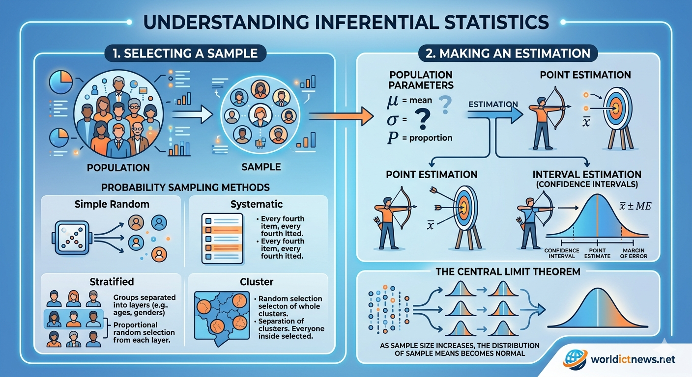
1. The Core Framework: Population vs. Sample

To understand how inferential statistics works, you must first master the distinction between a population and a sample.

• Population: The entire group of individuals, objects, or measurements that you want to study. For example, all registered voters in a country, or every smartphone manufactured by a factory in a year.

• Sample: A smaller, representative subset selected from the larger population. For example, 1,500 voters selected for a polling survey.

+------------------------------------------+

| POPULATION |
| (Parameters: Mean μ, SD σ) |
| |
| +----------------------------+ |
| | SAMPLE | |
| | (Statistics: Mean x̄, s) | |
| +----------------------------+ |
+------------------------------------------+

Parameters vs. Statistics

Data points change names depending on where they come from:

• Parameters: Numerical characteristics of a population (e.g., the true population mean, denoted by the Greek letter

  , or the population standard deviation, denoted by

  ). These are usually unknown because measuring the entire population is impossible.

• Statistics: Numerical characteristics of a sample (e.g., the sample mean, denoted as

  , or the sample standard deviation, denoted as

  ). These are calculated directly from your collected data.

The core objective of inferential statistics is to use known sample statistics to estimate unknown population parameters.

2. Sampling Methods: Building the Foundation

The validity of any statistical inference depends entirely on the quality of the sample. If a sample does not accurately reflect the diversity of the population, the resulting conclusions will be flawed. This flaw is known as sampling bias.

Sampling methods are broadly divided into two categories: probability sampling and non-probability sampling.

Probability Sampling Methods

In probability sampling, every member of the population has a known, non-zero chance of being selected. This category is the gold standard for inferential statistics because it minimizes bias and allows for mathematical calculations of error.

1. Simple Random Sampling (SRS)

Every individual in the population has an equal chance of selection.

• How it works: Assign a number to every individual and use a random number generator to pick the sample.

• Example: Putting 100 employee names into a digital hat and drawing 10.

• Pros & Cons: Highly objective and easy to explain, but can be logistical nightmares for massive populations.

2. Systematic Sampling

Members are selected at regular, predetermined intervals.

• How it works: Choose a random starting point, then select every

  -th individual from a ordered list (where

  ).

• Example: Selecting every 20th car that rolls off an assembly line.

• Pros & Cons: Simpler and faster than SRS. However, if the population list has a hidden repeating pattern (periodicity), the sample will be highly biased.

3. Stratified Sampling

The population is split into distinct, non-overlapping subgroups based on shared traits, called strata.

• How it works: Group the population by traits like age, gender, or income. Then, draw a random sample from each subgroup proportional to its size in the real population.

• Example: If a university is 60% undergraduate and 40% postgraduate, a stratified sample of 100 students will randomly pick exactly 60 undergraduates and 40 postgraduates.

• Pros & Cons: Ensures minority groups are fairly represented, increasing overall accuracy. The downside is that identifying and sorting individuals into clear strata requires deep prior knowledge of the population.

4. Cluster Sampling

The population is divided into naturally occurring groups, called clusters, typically based on geography or organization.

• How it works: Instead of selecting individual people, you randomly select entire clusters and survey everyone inside those chosen clusters.

• Example: To study high school students in a state, randomly select 10 school districts (clusters) and interview every student in those 10 districts.

• Pros & Cons: Highly cost-effective and practical for large geographical areas. However, people within the same cluster often share similar views or traits, which can make the sample less representative than an SRS of the same size.

Non-Probability Sampling Methods

In non-probability sampling, elements are chosen based on convenience, judgment, or specific criteria, meaning not everyone has a chance to be selected. While easier and cheaper, these methods cannot be used to make rigorous statistical inferences because they introduce heavy bias.

• Convenience Sampling: Choosing individuals who are easiest to reach (e.g., interviewing people walking past you at a mall).

• Purposive (Judgmental) Sampling: The researcher uses their personal expertise to handpick a sample they believe fits the study's specific goals.

• Snowboard / Chain Sampling: Existing research participants recruit future participants from among their acquaintances (useful for hard-to-reach populations like underground subcultures).

• Quota Sampling: Setting a specific target number of people who meet certain criteria (e.g., "find 50 men and 50 women"), but filling those spots using convenience methods rather than random selection.

3. The Central Limit Theorem (CLT): The Mathematical Bridge

Before moving from sampling to estimation, we must look at the mathematical engine driving inferential statistics: the Central Limit Theorem (CLT).

Imagine taking a random sample of 30 people from a city, calculating their average height, and plotting it on a graph. Now imagine doing this 10,000 times. You would create a distribution of thousands of different sample means. This distribution is called the sampling distribution of the mean.

The Central Limit Theorem states that:

1. Normal Shape: If your sample size (

   ) is sufficiently large (usually

   ), the sampling distribution of the mean will look like a bell-shaped curve (normal distribution). This remains true even if the underlying population distribution is completely skewed or irregular.

2. Center: The average of all your sample means will exactly equal the true population mean (

   ).

3. Spread (Standard Error): The spread of these sample means is called the Standard Error (

   ). It measures how much sample means fluctuate from sample to sample. It is calculated as:
   

   (Where

   is the population standard deviation and

   is the sample size).

The Central Limit Theorem is incredibly powerful. It proves that as your sample size grows larger, your sample mean becomes a highly reliable tracker of the true population mean.

4. Estimation: Finding the True Value

Once you have gathered a clean, random sample, you can use estimation to predict the true, hidden population parameters. Estimation is split into two strategies: Point Estimation and Interval Estimation.

Point Estimation

A point estimate uses a single calculated number from your sample to serve as the best guess for the population parameter.

• The sample mean (

  ) is the point estimate for the population mean (

  ).

• The sample proportion (

  ) is the point estimate for the population proportion (

  ).

The Flaw of Point Estimates: While simple, point estimates are almost never 100% accurate. If your sample mean for employee satisfaction is 7.4 out of 10, it is highly unlikely the true population average is exactly 7.40000. It might be 7.3 or 7.5. A point estimate gives you a target, but it fails to communicate the margin of error or how confident you are in that number.

Interval Estimation (Confidence Intervals)

To fix the limitations of a point estimate, statisticians prefer Interval Estimation. This approach builds a range of plausible values around your point estimate, known as a Confidence Interval (CI).

A confidence interval is structured as:

Understanding the Confidence Level

A confidence interval is always tied to a confidence level (usually 95% or 99%).

If you calculate a 95% Confidence Interval, it does not mean there is a 95% probability that the true population parameter sits inside that specific range. Instead, it means: "If we repeat this study with new random samples 100 times, 95 of the resulting intervals we calculate will successfully capture the true population parameter."

Calculating a Confidence Interval for a Population Mean (

)

The exact formula depends on whether you know the true population standard deviation (

).

Scenario A: When

is known (Using the Z-Distribution)

(Where

is the critical value from the standard normal distribution based on your confidence level).

• For a 95% confidence level, the

  -value is 1.96.

• For a 99% confidence level, the

  -value is 2.58.

Scenario B: When

is unknown (Using the t-Distribution)
In the real world, you almost never know the population standard deviation (

). When it is missing, you must swap it out for your sample standard deviation (

) and use the Student's t-distribution instead of the standard Z-distribution.

(Where

represents degrees of freedom, calculated as

).

The

-distribution looks similar to a normal distribution but has thicker tails. This shape accounts for the extra uncertainty that comes from estimating both the mean and the standard deviation at the same time. As your sample size (

) grows larger, the

-distribution flattens out until it matches the standard

-distribution.

Visual Comparison of Distributions:
Normal (Z) : _..---.._ (Thinner tails, higher peak)
t-dist (df=5): .' _..._ '. (Thicker tails, handles uncertainty)

5. Practical Example: Estimating Customer Spending

Let’s apply these theoretical steps to a practical business scenario.

The Problem

An e-commerce retailer wants to find the average amount of money spent per transaction on their website over the last year. They have millions of transactions, making it too slow and expensive to pull and clean the entire database. They decide to use inferential statistics.

Step 1: Sampling

The retailer extracts an automated Simple Random Sample of

transactions from the past year. Because the sample size is greater than 30 (

), the Central Limit Theorem applies, allowing them to proceed with confidence.

Step 2: Calculate Sample Statistics

After running the numbers on the 100 sampled transactions, they find:

• Sample mean spending (

  ): $85.00

• Sample standard deviation (

  ): $20.00

Step 3: Choose the Interval Model

Because the true population standard deviation (

) is unknown, they must use the

-distribution with degrees of freedom:

Looking at a standard

-table for a 95% confidence level with 99 degrees of freedom, the critical value is roughly:

Step 4: Compute the Margin of Error (MoE)

The margin of error is approximately $3.97.

Step 5: Build and Interpret the Interval

Conclusion: The retailer can state with 95% confidence that the true average spend across all millions of transactions falls somewhere between $81.03 and $88.97.

Summary of Key Formulas and Concepts

Conclusion

Inferential statistics changes data analysis from a passive backward glance into a forward-looking predictive tool. By understanding how to select an unbiased, random probability sample, you build a dependable foundation. By layering the Central Limit Theorem and interval estimation over that sample, you can extract deep insights about massive, complex populations using minimal data.

Whether you are optimizing factory operations, tracking public opinion trends, or launching a new business project, mastering these foundational techniques protects you from relying on guesswork, letting you base your decisions on mathematically sound conclusions