Calculating Descriptive Statistics for Grouped Data Using PSPP

Master Guide: Calculating Descriptive Statistics for Grouped Data Using PSPP.

Introduction

In data analysis, we often encounter datasets where individual raw scores are unavailable. Instead, the data is pre-arranged into intervals, ranges, or categories. This format is known as grouped data. Grouped data is highly efficient for summarizing massive datasets, tracking frequency distributions, and understanding demographic spreads. However, analyzing grouped data requires a fundamentally different statistical approach than analyzing unorganized raw data.

To analyze this data without expensive software licenses, researchers turn to PSPP. PSPP is a powerful, open-source alternative to IBM SPSS. It replicates the SPSS user interface and syntax, making high-level statistical analysis accessible to everyone.

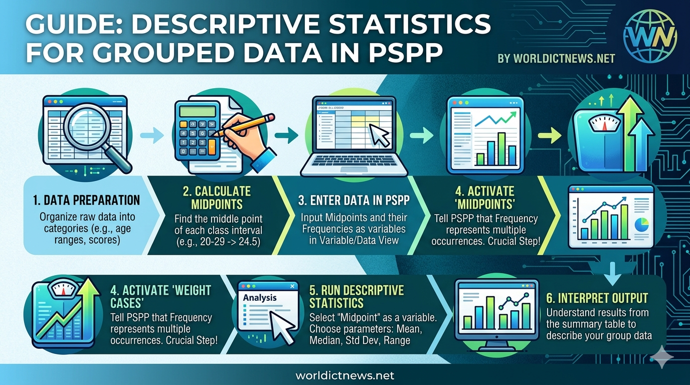
This comprehensive article provides a step-by-step procedure for calculating descriptive statistics for grouped data using PSPP. You will learn how to structure your dataset, apply essential statistical adjustments, and interpret your output data effectively.

1. Understanding Descriptive Statistics for Grouped Data

When dealing with ungrouped data, computing the mean, median, or standard deviation is straightforward. You simply add up the scores or look for the exact middle value. With grouped data, individual identities are lost inside class intervals (e.g., ages 20–29, 30–39).

To calculate statistics for grouped data, we must work with two primary components:

• Class Midpoints (\(X_{m}\)): The exact middle value of a class interval. This serves as the proxy value for all individual scores contained within that group.

• Frequencies (\(f\)): The number of observations or participants falling inside that specific interval.

Statistical Adjustments in PSPP

Software packages like PSPP are naturally built to calculate descriptive statistics from individual case rows. If you enter grouped data into PSPP normally, the software will read your frequencies as single, independent data points rather than group multipliers. To fix this, we must use a critical feature called Weight Cases. This instructs PSPP to treat your frequency column as a scale multiplier, ensuring your mean, variance, and standard deviation calculations are mathematically accurate for the total population size (\(N = \sum f\)).

2. Preparing and Formatting Grouped Data for PSPP

Before launching PSPP, you must structure your grouped data correctly. Let us look at a practical sample scenario: analyzing the monthly operational costs of 50 small tech startups.

Step 1: Calculate the Class Midpoints Manually

Standard statistical software cannot natively process a text range (like "$1,000 – $2,000") as a mathematical value. You must calculate the midpoint for each interval before data entry.

\(\text{Midpoint\ }(X_{m})=\frac{\text{Lower\ Limit}+\text{Upper\ Limit}}{2}\)

• For Interval 1: \((1000 + 2000) / 2 = \mathbf{1500}\)

• For Interval 2: \((2001 + 3000) / 2 = \mathbf{2500.5}\) (Rounded to 2501 for ease)

• For Interval 3: \((3001 + 4000) / 2 = \mathbf{3500.5}\) (Rounded to 3501)

• For Interval 4: \((4001 + 5000) / 2 = \mathbf{4501}\)

Step 2: Set Up Your Cleaned Data Table

Your adjusted table, ready for software input, will look like this:

3. Step-by-Step Data Entry in PSPP

With your midpoints calculated, it is time to input this information into PSPP.

Step 1: Define the Variables

1. Launch PSPP.

2. Look at the bottom-left corner of the interface and click on the Variable View tab.

3. In the first row under the Name column, type Midpoint and press Enter.

4. In the second row under the Name column, type Frequency and press Enter.

5. Keep the Type set to Numeric for both variables.

6. Set the Decimals column to 0 for clean numerical viewing.

7. Under the Label column, provide descriptive definitions for clarity:

   • For Midpoint, type: Estimated Class Midpoint (USD)

   • For Frequency, type: Number of Startup Observations

Step 2: Populate the Dataset

1. Switch to the Data View tab at the bottom-left corner of the screen.

2. You will now see two columns labeled Midpoint and Frequency.

3. Carefully type your calculated data matrix into the rows:

   • Row 1: 1500 under Midpoint | 8 under Frequency

   • Row 2: 2501 under Midpoint | 15 under Frequency

   • Row 3: 3501 under Midpoint | 18 under Frequency

   • Row 4: 4501 under Midpoint | 9 under Frequency

4. The Critical Step: Weighting Cases in PSPP

If you run descriptive statistics right now, PSPP will assume you only have 4 data points (1500, 2501, 3501, and 4501). It will completely ignore the fact that the number 3501 actually represents 18 different startups. You must activate case weighting to fix this.

Step-by-Step Activation via Graphical Interface (GUI)

1. Go to the top menu bar and click on Data.

2. Scroll to the bottom of the drop-down menu and select Weight Cases...

3. A new dialog box will appear. By default, the option Do not weight cases is selected.

4. Click the radio button next to Weight cases by.

5. Select your variable Frequency [Number of Startup Observations] from the left-hand asset list.

6. Click the pointing arrow button (\(\rightarrow \)) to move it into the Frequency Variable destination box.

7. Click OK.

Verification

Look closely at the bottom-right status bar of your main PSPP window. You should now see an indicator that reads "Weight on". This confirms that all subsequent operations will process your frequency column as a mathematical distribution multiplier (\(N=50\)).

5. Running the Descriptive Statistics Procedure

With your data structured and weighted, you can now generate your descriptive summary.

Step 1: Navigate to the Descriptives Dialog Box

1. Click on Analyze in the top menu header.

2. Hover your mouse over Descriptive Statistics.

3. Select Descriptives... from the side-context menu.

Step 2: Select Variables and Target Parameters

1. A dialog box titled Descriptives will open.

2. Select your variable Midpoint [Estimated Class Midpoint (USD)] from the left list.

3. Click the pointing arrow button (\(\rightarrow \)) to move it into the Variables target window.
   (Note: Do not add the Frequency variable here. Its job as a weight factor is already running silently in the background).

4. Look at the Statistics checkboxes located at the bottom of the dialog box. Select your required parameters:

   • Mean (Calculates the group average)

   • Std. deviation (Measures the spread of your data)

   • Minimum & Maximum (Displays your lowest and highest midpoints)

   • Variance (Measures the statistical dispersion)

   • Sum (Provides total accumulative financial volume)

5. Click OK.

6. Alternative Method: Executing via PSPP Syntax

If you prefer using command line inputs or need to document reproducible workflows for academic research, you can run this entire operation using PSPP Syntax.

1. Go to File \(\rightarrow \) New \(\rightarrow \) Syntax.

2. Paste the following explicit block of code into the blank workspace:

spss

* Step 1: Weight the dataset by the frequency count.
WEIGHT BY Frequency.

* Step 2: Run the descriptive statistics command on the midpoints.
DESCRIPTIVES
/VARIABLES=Midpoint
/STATISTICS=MEAN STDDEV MIN MAX VARIANCE SUM.

Use code with caution.

3. Highlight the code text using your mouse.

4. Go to the top menu and select Run \(\rightarrow \) Selection.

7. Interpreting the Output Data

Once processed, the PSPP Output Viewer window will automatically pop open to display a clean summary table. Let's analyze what your output results mean.

Descriptive Statistics
========================
Variable | N | Min | Max | Mean | Std Dev
---+-----+-------+-------+---------+--------
Estimated Class Midpoint (USD) | 50 | 1500 | 4501 | 3161.00 | 961.42
Valid N (listwise) | 50 | | | |
=========================

Explaining the Metrics

• N (Valid Observations): The system displays 50. This proves the Weight Cases feature worked perfectly. It successfully combined the frequencies (\(8+15+18+9\)) rather than treating the data as just 4 separate lines.

• Minimum and Maximum: Displays 1500 and 4501. These values represent the lowest and highest midpoint values calculated in your pre-processing phase.

• Mean: Displays 3161.00. This tells you that the average operational cost for a startup in this sample group is approximately $3,161.00.

• Standard Deviation: Displays 961.42. This indicates that most individual startup operational costs deviate from our central mean of $3,161 by roughly $961.42. A higher value suggests widely diverse costs across the industry, while a lower value implies consistent, predictable operational costs.

8. Common Pitfalls and Troubleshooting

To keep your research accurate, avoid these common mistakes when using PSPP:

• Forgetting to Apply Case Weights: If your output window displays an \(N\) value equal to your number of category rows (e.g., \(N=4\) instead of \(N=50\)), you forgot to activate the Weight Cases tool. Return to Data -> Weight Cases and re-apply the frequency variable.

• Failing to Clear Weights for Next Projects: The "Weight Cases" setting stays turned on until you manually turn it off. If you start a new analysis with a different dataset in the same session, it will corrupt your new data calculations. Always turn it off when finished by navigating to Data -> Weight Cases and selecting Do not weight cases.

• Using Non-Numeric Scale Values: Ensure your Midpoint column is categorized strictly as a Numeric variable type. If it is accidently set to String, it will trigger a fatal error, or the variable will not show up in the descriptive analysis asset list.

Conclusion

Calculating descriptive statistics for grouped data in PSPP is an efficient process once you master data formatting and case weighting. This workflow allows you to extract clean mean values, group variances, and standard deviations from condensed secondary data reports.

By applying these structural steps, you can confidently turn raw frequency metrics into clear, professional research summaries.