Data Science Lifecycle: From Collection to Deployment

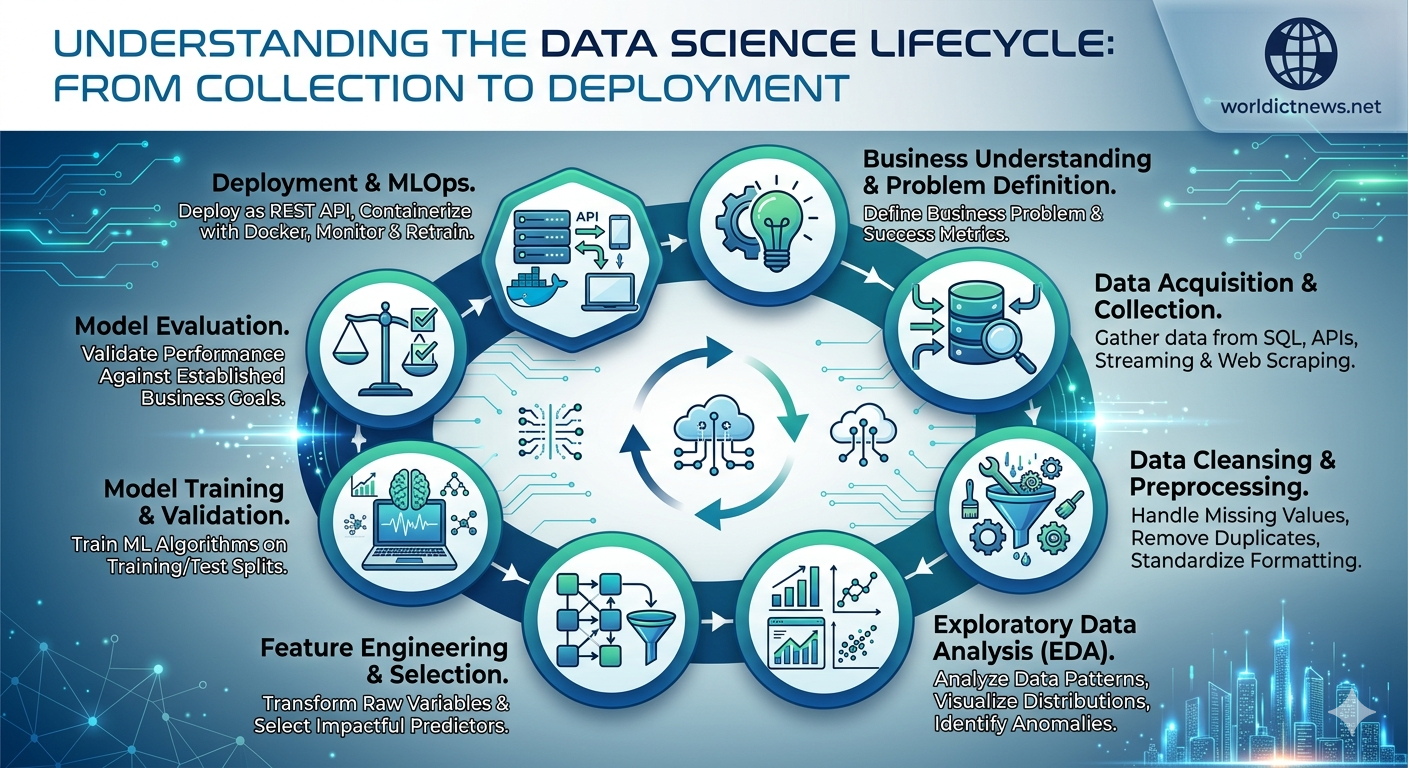
Understanding the Data Science Lifecycle: From Collection to Deployment.

In the modern digital economy, data is frequently described as the new oil. However, raw data, much like unrefined petroleum, holds little inherent value. The true power of data lies in an organization's ability to extract actionable insights, build predictive systems, and automate decision-making processes. To transform chaotic datasets into strategic business assets, data professionals rely on a structured, iterative framework known as the Data Science Lifecycle.

The Data Science Lifecycle serves as a roadmap for executing complex data projects. It ensures that data initiatives align with commercial objectives, maintain statistical integrity, and culminate in stable production deployments. Whether you are building an AI-powered product recommendation engine or analyzing customer churn trends, following this end-to-end lifecycle is critical to avoiding project failure. This comprehensive guide details the foundational phases of the lifecycle—from initial data acquisition to final model deployment.

1. Business Understanding and Problem Definition

Every successful data science project begins not with code or algorithms, but with clear business objectives. Jumping directly into data collection without defining a specific problem is one of the leading causes of enterprise data project cancellation.

During this initial phase, data scientists collaborate closely with domain experts, product managers, and executive stakeholders to answer fundamental questions:

• What specific business problem are we trying to solve? (e.g., Reducing fraudulent financial transactions).

• What are the project constraints, timelines, and budget limitations?

• How will the success of the project be measured?

+-------------------------------------------------------------------+

| PROJECT METRIC ALIGNMENT |
| |
| Business Goal: Reduce Customer Churn |
| │ |
| ▼ |
| Data Science Metric: Optimize ROC-AUC / F1-Score for Fraud Class|
+-------------------------------------------------------------------+

This phase bridges the gap between commercial terminology and statistical metrics. For instance, if the business goal is to "improve customer retention," the data science team must translate this into a measurable modeling target, such as "building a binary classification model to predict which users have a high probability of canceling their subscription within the next 30 days."

2. Data Acquisition and Collection

Once the objective is established, the next step is gathering the raw material: data. Depending on the project scope, data can originate from a variety of sources, both internal and external to the enterprise.

Data collection strategies generally fall into three categories:

Internal Relational Databases

Most corporate data resides within structured transactional databases. Data engineers and data scientists use Structured Query Language (SQL) to extract historical customer records, sales transactions, and product inventories from systems like PostgreSQL, MySQL, or enterprise data warehouses like Snowflake and Google BigQuery.

Application Log Files and Streaming Data

For real-time applications, data is continuously ingested via event streams. For example, tracking user clicks on an e-commerce website or gathering sensor metrics from IoT devices requires streaming pipelines managed by tools like Apache Kafka or AWS Kinesis.

External APIs and Web Scraping

When internal data is insufficient, external datasets must be acquired. This involves programmatically pulling data via third-party Application Programming Interfaces (APIs), utilizing public datasets (such as those found on Kaggle or government repositories), or leveraging web scraping frameworks like Beautiful Soup and Scrapy to extract unstructured web text.

3. Data Cleansing and Preprocessing

Raw data is rarely clean. It is often riddled with missing values, duplicate entries, formatting inconsistencies, and statistical anomalies. Data cleansing—frequently called data wrangling—is the most time-consuming phase of the lifecycle, often consuming up to 70% to 80% of a data scientist's total workflow.

Raw Data ──► [ Deduplication ] ──► [ Imputation ] ──► [ Type Casting ] ──► Clean Data

Key preprocessing operations include:

Handling Missing Values

Data records frequently contain blank entries. Data scientists must decide whether to remove rows with missing attributes entirely or fill them using statistical estimation techniques known as imputation (e.g., replacing a missing age value with the column's mean or median).

Eliminating Duplicates and Corrupted Rows

System glitches can cause duplicate records or corrupt entries. Identifying and purging these anomalies ensures that machine learning models are not trained on skewed or incorrect inputs.

Data Type Standardizations

Data must be correctly formatted before mathematical processing. This involves converting string characters into numerical values, standardizing datetime fields across uniform time zones, and ensuring categorical elements (like "True/False" or "Yes/No") are parsed systematically.

4. Exploratory Data Analysis (EDA)

With clean data in hand, data scientists perform Exploratory Data Analysis (EDA). The objective of EDA is to explore the dataset's underlying structure, identify patterns, detect anomalies, and test hypotheses using visual and statistical summaries.

[ Histogram ] [ Scatter Plot ] [ Heatmap ]
Distribution Check Correlation Detection Multicollinearity Check

EDA typically leverages three core visualization techniques:

• Histograms and Box Plots: Used to examine the distribution of individual variables and isolate extreme values (outliers) that could distort future predictions.

• Scatter Plots: Utilized to map two distinct variables against one another, revealing hidden linear or non-linear correlations.

• Correlation Heatmaps: Used to analyze the linear relationships across all numerical columns simultaneously. This helps identify multicollinearity, a condition where two input features are highly correlated, potentially degrading the stability of certain machine learning models.

5. Feature Engineering and Selection

Feature engineering is the process of using domain knowledge to transform raw variables into more informative inputs (features) that enhance the predictive accuracy of machine learning models.

Feature Transformation Examples

• Temporal Extractions: Extracting specific data components from a single timestamp field, such as converting "2026-05-16 18:35:00" into categorical components like "Day of Week: Saturday" or "Hour: 18".

• One-Hot Encoding: Converting text-based categorical variables (such as a "Country" column containing values like "USA", "UK", or "Nigeria") into separate binary columns containing 0s and 1s, which algorithms can process mathematically.

• Feature Scaling: Normalizing numerical variables to sit within a uniform scale (e.g., between 0 and 1) using techniques like Min-Max Scaling or Standardization. This prevents features with large numeric scales (like annual income) from over-indexing against smaller scales (like age).

Feature Selection

Including too many variables can cause models to overfit, slow down training times, and increase computational costs. Feature selection algorithms help isolate the most important predictors while discarding redundant or irrelevant data columns.

6. Model Training and Validation

This phase is where predictive modeling takes place. Data scientists select appropriate machine learning algorithms based on the problem definition established in phase one.

Entire Dataset
├── Train Set (80%) ──► Train Model Adjusting Weights
└── Test Set (20%) ──► Evaluate Unseen Generalization

Algorithm Categories

• Regression Models: Used for predicting continuous numerical outputs (e.g., Linear Regression or Random Forest Regressors to predict housing prices).

• Classification Models: Used for predicting discrete categorical outputs (e.g., Logistic Regression, Support Vector Machines, or Gradient Boosting Classifiers to determine if an email is "Spam" or "Not Spam").

• Clustering Models: Unsupervised techniques used to group unlabelled data points based on geometric proximity (e.g., K-Means clustering for market segmentation).

Training and Testing Split

To ensure a model can generalize effectively to new data, the dataset is split into two parts: a Training Set (typically 80%) used to build the model, and a Testing Set (typically 20%) kept isolated. Evaluating the model against the testing set provides an unbiased assessment of its real-world performance.

7. Model Evaluation

Before a model is allowed to influence business operations, its performance must be validated against standardized metrics. Relying solely on basic "Accuracy" can be highly misleading, especially when dealing with unbalanced datasets.

Consider a fraud detection system where only 1% of transactions are actually fraudulent. A broken model that simply guesses "Not Fraud" for every transaction will technically achieve 99% accuracy, while failing completely at its actual objective. Data scientists rely on more robust evaluation metrics to measure true performance:

ACTUAL VALUES
True False
PREDICTED +--------+-----------+
VALUES | TP | FP | --> Precision = TP / (TP + FP)
+--------+-----------+

| FN | TN | --> Recall = TP / (TP + FN)
+--------+-----------+

• Precision: Measures the proportion of predicted positive instances that were actually correct. This is critical when false positives are expensive.

• Recall (Sensitivity): Measures the proportion of actual positive instances that the model successfully caught. This is vital in scenarios like medical diagnostics or fraud detection, where missing a true positive has severe consequences.

• F1-Score: The harmonic mean of Precision and Recall, providing a balanced metric for uneven datasets.

• ROC-AUC Score: Evaluates how well a classification model separates different classes across various decision thresholds.

8. Deployment and MLOps

The final phase of the Data Science Lifecycle moves the trained model out of the local development environment (like Jupyter Notebooks) and into a production ecosystem where apps and end-users can access it in real time. This transition falls under the domain of MLOps (Machine Learning Operations).

[ Local Notebook ] ──► [ Docker Container ] ──► [ REST API Endpoint ] ──► [ Web App ]

A standard deployment workflow follows these operational steps:

Containerization with Docker

The model files, code libraries, dependencies, and configuration settings are packaged together into a isolated Docker Container. This guarantees that the model runs identically regardless of whether it is hosted on a local testing laptop or an enterprise cloud cluster.

Exposing as a REST API

The containerized model is wrapped in a lightweight web framework like FastAPI or Flask and deployed as an active API endpoint. External applications can send data to this endpoint via JSON requests and receive live model predictions within milliseconds.

Production Infrastructure

API endpoints are scaled across cloud infrastructure using orchestration tools like Kubernetes, or serverless deployment pipelines like AWS SageMaker, Azure ML, or Google Vertex AI.

Continuous Monitoring and Drift Detection

Deploying a model is not a one-time event. Over time, real-world data distributions change, causing a drop in predictive accuracy—a phenomenon known as Model Drift or Data Drift. Production monitoring pipelines track incoming data and trigger automated retraining loops when performance dips below acceptable thresholds.

Conclusion

The Data Science Lifecycle is a structured, end-to-end framework that converts raw data into reliable, production-ready systems. Navigating from initial business alignment through cleansing, feature engineering, modeling, and MLOps deployment requires careful execution at every step. By adhering to this lifecycle, organizations can build robust analytics frameworks that add measurable, scalable value to their digital infrastructure.

Frequently Asked Questions (FAQ)

1. Why is Exploratory Data Analysis (EDA) important before machine learning?

EDA helps data scientists understand the underlying patterns, structure, and quality of a dataset before training models. Skipping EDA can lead to training algorithms on skewed data, missing critical feature correlations, or failing to identify outliers that distort predictive accuracy.

2. What is the difference between Precision and Recall?

Precision measures the accuracy of positive predictions (out of all examples predicted as positive, how many were true). Recall measures the model's ability to find all positive instances (out of all actual positive examples, how many were correctly caught).

3. What causes Model Drift in production environments?

Model Drift occurs when the real-world data an active model encounters shifts away from the historical data it was originally trained on. Changes in consumer behavior, macroeconomic trends, or system updates can alter data patterns, making older predictions less accurate over time.

4. What role does Docker play in the Data Science Lifecycle?

Docker standardizes model deployment by packaging code, runtime environments, and dependencies into an isolated container. This eliminates the "it works on my machine" problem, ensuring the model functions consistently across local machines, staging areas, and live cloud environments.

5. Why does data cleaning take up the majority of a project's timeline?

Real-world data is routinely collected from uncoordinated logs, user inputs, and legacy databases. Resolving missing values, fixing corrupted formats, and standardizing datatypes requires meticulous programmatic checks to avoid feeding low-quality data into machine learning models.