Introduction to Statistics for Data Science

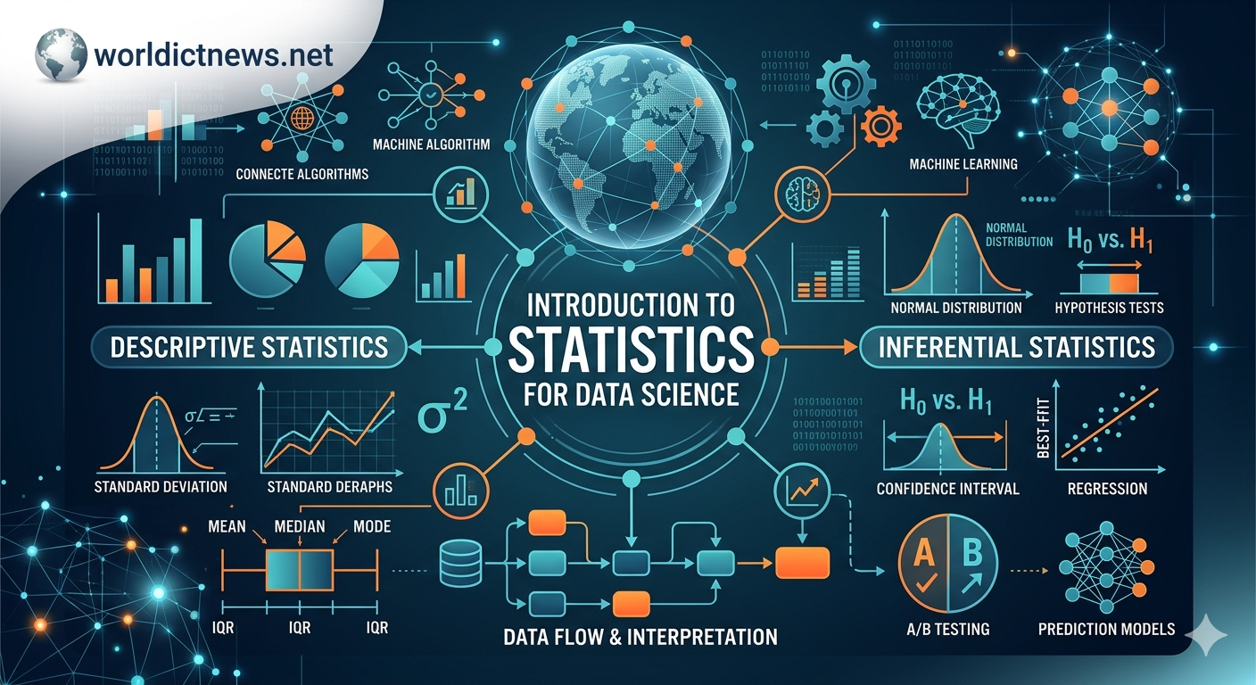
Introduction to Statistics for Data Science: The Foundational Language of Data.

In the modern technological landscape, data science is often romanticized through the lens of complex machine learning architectures, deep neural networks, and generative artificial intelligence. However, stripping away the algorithmic layers reveals that the core operating engine of data science is built entirely on statistics.

Data science is the practice of extracting actionable insights from data, and statistics is the formal language that allows us to do so accurately. Without a solid understanding of statistics, data scientists run the risk of mistaking random noise for meaningful patterns, building biased predictive models, and drawing flawed conclusions.

This comprehensive guide serves as an entry point into statistics for data science, mapping out the fundamental concepts—from basic summary metrics to advanced probabilistic frameworks—needed to turn raw variables into strategic assets.

Part I: The Two Pillars of Statistics

Statistical analysis is broadly divided into two primary disciplines: Descriptive Statistics and Inferential Statistics. A data scientist must master both to move from simply describing what has happened to predicting what will happen next.

┌────┐
│ STATISTICS FOR DATA SCIENCE │
└─┬──┘
│
┌──┴──┐
▼ ▼
┌───┐ ┌───┐
│ DESCRIPTIVE STATISTICS │ │ INFERENTIAL STATISTICS │
├─┤ ├─┤
│ • Central Tendency │ │ • Hypothesis Testing │
│ • Dispersion / Variance │ │ • Confidence Intervals │
│ • Shape of Distribution │ │ • Regression Modeling │
└───┘ └──┘

1. Descriptive Statistics

Descriptive statistics focus on summarizing and organizing a dataset so its core characteristics are immediately apparent. It acts as the initial step in Exploratory Data Analysis (EDA).

Measures of Central Tendency

These metrics help identify the "center" or typical value of a data distribution:

• Mean: The arithmetic average of all data points. It is highly sensitive to outliers.

• Median: The exact middle value when data points are sorted in ascending order. It is highly robust against skewed data.

• Mode: The most frequently occurring value in the dataset, which is useful for categorical variables.

Measures of Dispersion (Spread)

Understanding the spread of your data is just as vital as finding its center. Two datasets can have the exact same mean but entirely different distributions.

• Range: The difference between the highest and lowest values in a dataset.

• Variance (\(\sigma ^{2}\)): The average of the squared differences from the mean. It quantifies how much the data points drift from the center.

• Standard Deviation (\(\sigma \)): The square root of the variance. It translates the dispersion metric back into the original unit of measurement, making it highly interpretable.

• Interquartile Range (IQR): The distance between the 25th percentile (Q1) and the 75th percentile (Q3). Data scientists use IQR heavily to identify and isolate anomalies and outliers via boxplots.

Part II: Probability and Data Distributions

Data is rarely uniform. It takes on various shapes when plotted, and these shapes—known as distributions—dictate the mathematical assumptions a data scientist can make about their models.

Standard Normal Distribution (68-95-99.7 Rule)
|
. | .
. | .
. | .
. | .
_______.___.___.___.___________.___.___.___._______
-3σ -2σ -1σ μ 1σ 2σ 3σ

|___________|___________|
68%

|___________________|
95%

|_______________________________|
99.7%

1. The Normal (Gaussian) Distribution

The Normal Distribution is the cornerstone of classical statistics. It forms a perfectly symmetrical "bell curve" where the mean, median, and mode are all equal.

Data scientists rely on the Empirical Rule (68-95-99.7 Rule) to understand variables that follow this distribution:

• 68% of all data points fall within one standard deviation (\(\pm1\sigma\)) of the mean.

• 95% of all data points fall within two standard deviations (\(\pm2\sigma\)) of the mean.

• 99.7% of all data points fall within three standard deviations (\(\pm3\sigma\)) of the mean.

Many real-world phenomena—such as human heights, standardized test scores, and even the errors generated by machine learning models—naturally follow a normal distribution.

2. Other Key Distributions in Data Science

• Binomial Distribution: Measures the probability of a binary outcome (success/failure) across a fixed number of independent trials. It is used to analyze conversions, like whether a user will click an ad or close the tab.

• Poisson Distribution: Calculates the probability of a given number of events occurring within a fixed interval of time or space. It helps optimize systems like server traffic or customer queue lengths.

• Uniform Distribution: Occurs when all outcomes have an equal probability of happening, such as rolling a fair die or generating a random number within a specific range.

Part III: Inferential Statistics and Hypothesis Testing

Inferential statistics allows data scientists to take a small sample of data and draw conclusions about a much larger population. This is where business experimentation, such as A/B testing, derives its legitimacy.

1. The Central Limit Theorem (CLT)

The Central Limit Theorem is the foundational bridge between descriptive and inferential statistics. It states that if you take sufficiently large samples from any population, the distribution of the sample means will approach a normal distribution, regardless of the shape of the original population.

This theorem allows data scientists to make confident inferences about highly skewed population data using parametric models, provided the sample size is large enough (typically \(n \ge 30\)).

2. The Architecture of Hypothesis Testing

Hypothesis testing is a structured framework used to determine whether a specific data pattern occurred due to an actual cause or simply by random chance.

┌─────┐
│ HYPOTHESIS TESTING FRAMEWORK │
├───┬─────┤
│ NULL ($H_0$) │ ALTERNATIVE ($H_1$) │
├───┼──┤
│ • Status quo │ • The effect is real │
│ • No change or effect │ • Statistically meaningful │
│ • Observed by pure chance │ • Target of the experiment │
└──┴───┘

• Null Hypothesis (\(H_{0}\)): The default assumption that there is no significant difference or effect. Any observed change is due to random variance.

• Alternative Hypothesis (\(H_{1}\)): The statement you want to prove. It asserts that the observed difference is real and caused by a specific variable.

3. P-Values and Significance Levels (\(\alpha \))

To choose between the Null and Alternative hypotheses, data scientists look at the p-value:

• Significance Level (\(\alpha \)): The threshold for risk, typically set at \(0.05\) (\(5\%\)). It represents the probability of rejecting the null hypothesis when it was actually true (a Type I error).

• The Decision Rule: If the computed p-value is less than or equal to \(\alpha \) (\(p \le 0.05\)), the result is considered statistically significant. You reject the Null Hypothesis and accept the Alternative. If the p-value is higher, you fail to reject the null hypothesis.

Part IV: Quantifying Relationships (Correlation vs. Causation)

A significant portion of predictive modeling involves understanding how different variables interact with one another.

1. Correlation Coefficient (\(r\))

Pearson’s correlation coefficient measures the linear strength and direction of the relationship between two continuous variables. The metric ranges strictly between \(-1\) and \(+1\):

• \(+1\): A perfect positive linear relationship (as \(X\) increases, \(Y\) increases proportionally).

• \(0\): Absolute zero linear relationship between the variables.

• \(-1\): A perfect negative linear relationship (as \(X\) increases, \(Y\) decreases proportionally).

Positive Correlation (+1) Negative Correlation (-1)
* * *
* * * *
* * * *
* * *

2. The Causation Fallacy

One of the most vital rules in data science is that correlation does not imply causation. Two variables can follow identical mathematical trends due to an unmeasured third factor (a confounding variable) or pure coincidence.

For example, ice cream sales and sunburn rates are highly correlated, but buying ice cream does not cause a sunburn. Both are driven by a third variable: hot summer weather. Data scientists must use randomized controlled experiments to prove actual causality.

Part V: Statistics in Practical Machine Learning

Statistical principles directly govern how machine learning models learn, make predictions, and handle errors.

1. The Bias-Variance Tradeoff

When training a predictive model, statistics helps us balance two types of errors:

• Bias: Errors caused by oversimplified assumptions in the model. High bias leads to underfitting, where the model fails to capture the underlying patterns in the training data.

• Variance: Errors caused by overcomplicating the model. High variance leads to overfitting, where the model learns the training data's random noise so perfectly that it fails to generalize to fresh, unseen data.

┌──────┐
│ THE MODEL FIT SPECTRUM │
├──┬──┬──┤
│ UNDERFITTING │ GOOD FIT │ OVERFITTING │
├──┼───┼──┤
│ • High Bias │ • Optimal Balance │ • High Variance│
│ • Low Variance │ • Low Total Error │ • Low Bias │
│ • Missing trends │ • Generalizes well│ • Learns noise │
└───┴───┴───┘

2. Feature Selection and Dimensionality

In big data environments, datasets often contain hundreds of columns (features). Data scientists use statistical techniques like Variance Inflation Factors (VIF), Chi-Square tests, and Principal Component Analysis (PCA) to eliminate redundant features. This process streamlines datasets, speeds up model training times, and prevents errors associated with multicollinearity.

Conclusion: Elevating Data Science Beyond Algorithms

Algorithms provide machine learning models with their muscle, but statistics provides them with their sight. No matter how advanced your programming pipelines become, the validity of your data products relies on foundational statistics.

By understanding how data distributions behave, implementing rigorous hypothesis tests, and recognizing the spread and limitations of your metrics, you ensure that your data science conclusions are mathematically sound, highly repeatable, and reliable in production environments.