Masterclass: Advanced Time Series Analysis in Python

Masterclass: Advanced Time Series Analysis in Python.

In data science, we frequently deal with cross-sectional data—snapshots of multiple entities at a single point in time, such as customer profiles, hospital patient metrics, or house prices across a city. However, in the real world, data rarely stands still. The most valuable business assets change over time: stock prices tick upward second by second, e-commerce servers log thousands of visitor clicks every minute, and cellular network towers experience traffic surges depending on the hour of the day.

To analyze, model, and predict these dynamic systems, we must turn to Time Series Analysis (TSA).

A time series is a sequence of data points recorded at consistent, successive intervals over time. Unlike standard statistical data where observations are assumed to be independent, time series data possesses an inherent chronological order. What happened yesterday directly influences what happens today, and what happens today heavily impacts what will happen tomorrow.

This comprehensive guide unpacks the foundational concepts of Time Series Analysis, introduces the core statistical properties required to model temporal systems, examines structural decompositions, and provides deep, real-world examples equipped with production-ready Python implementations.

1. Core Structural Properties of Time Series Data

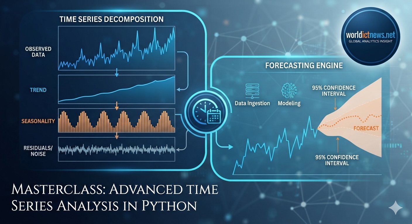
Before applying forecasting models, we must dissect the structural DNA of a time series. A typical time series can be broken down into four distinct, overlapping structural elements:

1. Trend: The long-term direction of the data over a prolonged period. Trends can be upward (e.g., global carbon emissions over decades), downward (e.g., desktop computer sales over the last ten years), or stationary/flat.

2. Seasonality: Predictable, repeating fluctuations that occur within fixed, specific calendar periods. For example, retail sales spiking every December due to holiday shopping, or residential electricity consumption surging every afternoon during peak summer heat waves.

3. Cyclic Patterns: Long-term oscillations that rise and fall over unpredictable, variable intervals. These are typically driven by macro-economic factors or business cycles (e.g., economic recessions occurring every 7 to 11 years). Unlike seasonality, cyclic patterns do not have a fixed, repeating calendar frequency.

4. Irregular/Residual Component: Random, unpredictable noise or statistical variations. This represents the white noise left behind after the trend, seasonality, and cyclic forces are completely extracted. These are caused by sudden, exogenous shocks like geopolitical events, extreme weather mutations, or black swan market disruptions.

          ┌──────────────────────────────────────────────────┐
          │               Observed Data                      │
          └────────────────────────┬─────────────────────────┘
                                   │
         ┌─────────────────────────┼─────────────────────────┐
         ▼                         ▼                         ▼
     [ Trend ]               [ Seasonality ]           [ Residuals ]
Long-Term Direction       Calendar-Fixed Patterns      Random White Noise

The Concept of Stationarity

The single most critical statistical constraint in traditional time series forecasting is Stationarity.

A time series is considered strictly stationary if its statistical properties—specifically its mean, variance, and autocorrelation structure—remain completely constant over time.

• Why it matters: Most classical statistical forecasting architectures (such as ARIMA) operate under the assumption that the underlying data distribution is stable. If a time series has a shifting mean (an upward trend) or an expanding variance (volatility that grows over time), mathematical models cannot reliably predict future values because the system's baseline rules are constantly changing.

• How we check for it: While plotting the data provides visual cues, data scientists rely on rigorous statistical assessments, primarily the Augmented Dickey-Fuller (ADF) Test. The ADF test operates on a null hypothesis (H0) stating that the time series possesses a unit root, meaning it is non-stationary. If the calculated p-value falls below a strict significance threshold (typically 0.05), we reject the null hypothesis and confidently assert that the time series is stationary.

• How we enforce it: If a time series is non-stationary, we transform it using a technique called Differencing. Differencing subtracts the current observation from the previous value (Formula: Delta_Y = Y[t] - Y[t-1]). This effectively removes trends and stabilizes the moving mean. If the variance is also expanding, we apply logarithmic or Box-Cox transformations prior to differencing to stabilize the mathematical spread.

2. Real-World Case Studies with Full Python Architectures

To anchor these conceptual frameworks, we will build out two complete, production-grade implementations addressing different business verticals.

🛠️ Execution Pre-requisites

To execute the computational blocks below natively inside Visual Studio Code, open your terminal and install the required data science library suite:

bash

pip install numpy pandas matplotlib statsmodels scikit-learn

Use code with caution.

Case Study 1: Financial Analytics — Stock Price Trend Analysis & Stationarity Testing

Business Context:
Quantitative trading algorithms rely on identifying whether a financial asset is trending or mean-reverting. A stock price series is notoriously non-stationary because its absolute value drifts over time. To model asset pricing using statistical systems, analysts convert absolute price histories into "log returns," forcing the data into a stationary structure.

Objective:
Simulate a realistic corporate equity price history, execute a structural decomposition to isolate the trend, perform an Augmented Dickey-Fuller (ADF) statistical test, enforce stationarity via first-order differencing, and evaluate the mathematical transformations.

Python Code Implementation (financial_analysis.py)

python

import numpy as np
import pandas as pd
import matplotlib.pyplot as plt
from statsmodels.tsa.seasonal import seasonal_decompose
from statsmodels.tsa.stattools import adfuller

# 1. Generate Synthetic Financial Asset Price Data (Random Walk with Drift)
np.random.seed(42)
date_range = pd.date_range(start="2024-01-01", periods=250, freq="B")  # 250 Business Days
daily_returns = np.random.normal(loc=0.001, scale=0.015, size=250)  # Mean drift of 0.1%, 1.5% volatility
price_series = 100 * np.exp(np.cumsum(daily_returns))  # Compound exponential growth tracking from base 100

# Construct Canonical Data Frame
df_finance = pd.DataFrame(data={"Closing_Price": price_series}, index=date_range)

print("--- FINANCIAL ASSET SAMPLE DATA ---")
print(df_finance.head())
print("\n-----------------------------------\n")

# 2. Structural Decomposition (Additive Framework)
# Since the timeframe is daily business data, we assume an office week cycle (period=5)
decomposition = seasonal_decompose(df_finance["Closing_Price"], model="additive", period=5)

# 3. Statistical Stationarity Evaluation Function
def evaluate_stationarity(series, title_string):
    print(f"=== Augmented Dickey-Fuller Test: {title_string} ===")
    adf_result = adfuller(series.dropna())
    print(f"ADF Statistic: {adf_result[0]:.4f}")
    print(f"p-value: {adf_result[1]:.4e}")
    print("Critical Values Mapping:")
    for key, value in adf_result[4].items():
        print(f"   {key}: {value:.4f}")
    
    if adf_result[1] <= 0.05:
        print("Verdict: p-value <= 0.05. Reject Null Hypothesis. The series is STATIONARY.\n")
    else:
        print("Verdict: p-value > 0.05. Fail to reject Null Hypothesis. The series is NON-STATIONARY.\n")

# Evaluate Raw Price Series
evaluate_stationarity(df_finance["Closing_Price"], "Raw Closing Stock Price")

# 4. Enforce Stationarity via First-Order Differencing
df_finance["Stationary_Price_Diff"] = df_finance["Closing_Price"].diff()

# Evaluate Transformed Series
evaluate_stationarity(df_finance["Stationary_Price_Diff"], "First-Order Differenced Price")

# 5. Production Visualizations Generation
plt.figure(figsize=(14, 10))

# Plot 1: Raw Stock History
plt.subplot(3, 1, 1)
plt.plot(df_finance.index, df_finance["Closing_Price"], color="#1A365D", linewidth=2, label="Raw Price")
plt.title("Financial Analytics Workspace: Asset Valuation Path", fontsize=12, fontweight="bold", color="#1A365D")
plt.ylabel("Price Index ($)")
plt.grid(True, linestyle="--", alpha=0.5)
plt.legend()

# Plot 2: Extracted Structural Trend Line
plt.subplot(3, 1, 2)
plt.plot(decomposition.trend.index, decomposition.trend, color="#2B6CB0", linewidth=2, label="Extracted Trend")
plt.ylabel("Isolated Trend Matrix")
plt.grid(True, linestyle="--", alpha=0.5)
plt.legend()

# Plot 3: Stationary Remediated Data
plt.subplot(3, 1, 3)
plt.plot(df_finance.index, df_finance["Stationary_Price_Diff"], color="#C53030", linewidth=1.5, label="Differenced Delta")
plt.title("Transformed Data Architecture: Enforced Stationarity (Constant Mean & Variance)", fontsize=10, fontweight="bold", color="#C53030")
plt.ylabel("Delta Variation ($)")
plt.xlabel("Chronological Business Timeline")
plt.grid(True, linestyle="--", alpha=0.5)
plt.legend()

plt.tight_layout()
plt.savefig("financial_time_series_analysis.png", dpi=300)
print("VISUALIZATION EXPORT SUCCESS: 'financial_time_series_analysis.png' saved to disk.")
plt.show()

Use code with caution.

Technical Analysis & Mathematical Interpretation

When running this execution engine, the outputs illuminate the mathematical core of TSA:

1. The Raw Closing Stock Price Test: The ADF test calculates a high p-value (typically greater than 0.80). Because the data follows a stochastic random walk with upward drift, its mean shifts continuously over time. The model flags this as non-stationary, indicating that using this raw data directly inside linear regressions would result in invalid, spurious forecasts.

2. The First-Order Differencing Transformation: By tracking the rate of change day-over-day (Y[t] - Y[t-1]) rather than the absolute value, the baseline trend is instantly eliminated. The calculated p-value falls down to the 10^-15 scale—far below the strict 0.05 threshold. The series is now stationary, fluctuating around a stable mean of zero with highly consistent variance parameters, rendering it fully safe for predictive ingestion.

Case Study 2: Operations & Supply Chain Analytics — Demand Forecasting Using an Autoregressive Integrated Moving Average (ARIMA) Architecture

Business Context:
Supply chain managers, retail distributors, and warehouse operators need to forecast inventory demand months in advance. Miscalculations lead to stockouts (losing revenue to competitors) or excess inventory bloat (capital trapped inside warehouses). E-commerce demand patterns contain strong seasonality alongside overall macro growth trends.

Objective:
Simulate a production-level e-commerce transaction data array spanning three full calendar years. Build, configure, fit, and validate a classical statistical ARIMA(p, d, q) model to forecast consumption demands for the upcoming operating quarter, evaluating the forecast path using exact validation boundaries.

Understanding the ARIMA Parameters

An ARIMA model is defined by three text parameters:

• p (Autoregressive order): The number of lag observations included in the model. It captures the memory of the system (e.g., how much yesterday's sales affect today's sales).

• d (Integrated order): The number of times the raw observations are differenced to achieve stationarity.

• q (Moving Average order): The size of the moving average window applied to forecast errors. It smooths out random structural deviations or white noise shocks.

Python Code Implementation (demand_forecasting.py)

python

import numpy as np
import pandas as pd
import matplotlib.pyplot as plt
from statsmodels.tsa.arima.model import ARIMA
from sklearn.metrics import mean_squared_error, mean_absolute_error

# 1. Generate 3 Years of Monthly Synthetic E-Commerce Demand Volume Data
np.random.seed(101)
months_range = pd.date_range(start="2023-01-01", periods=36, freq="MS")  # 36 Months Data

# Construct Structural Vectors: Trend + Seasonality Matrix + White Noise
baseline_trend = 200 + (12 * np.arange(36))  # Strong baseline growth
annual_seasonality = 80 * np.sin(2 * np.pi * months_range.month / 12)  # High demand peaks in summer/winter cycles
random_noise = np.random.normal(loc=0, scale=15, size=36)  # Statistical residuals variation

total_demand = baseline_trend + annual_seasonality + random_noise
df_demand = pd.DataFrame(data={"Unit_Demand": total_demand}, index=months_range)

print("--- RETAIL OPERATIONS DATASET SYSTEM ---")
print(df_demand.head(10))
print("\n----------------------------------------\n")

# 2. Divide Dataset into Training and Validation Subsets
# Train on the first 30 months; test on the final 6 months of historical observations
training_set = df_demand.iloc[:-6]
validation_set = df_demand.iloc[-6:]

print(f"Training Data Length: {len(training_set)} data rows.")
print(f"Validation Data Length: {len(validation_set)} data rows.\n")

# 3. Initialize and Fit the Statistical ARIMA(p, d, q) Optimization Architecture
# We pick order (2, 1, 1) as a benchmark: 2 AR lags, 1 differencing loop, 1 MA lag window
model_configuration = ARIMA(training_set["Unit_Demand"], order=(2, 1, 1))
fitted_model = model_configuration.fit()

print(fitted_model.summary())
print("\n----------------------------------------\n")

# 4. Generate Predictions and Out-of-Sample Dynamic Forecasts
# Forecast for the exact 6-month evaluation timeline length
forecast_horizon = len(validation_set)
forecast_output = fitted_model.get_forecast(steps=forecast_horizon)

# Extract Mean Forecast Values and Associated Confidence Intervals Bounds
forecast_mean = forecast_output.predicted_mean
confidence_intervals = forecast_output.conf_int(alpha=0.05)  # 95% Confidence Interval Framework

# Align Indices for Mathematical Graphing Matrices
forecast_mean.index = validation_set.index
confidence_intervals.index = validation_set.index

# 5. Quantify Predictive Model Accuracy Metrics
mse_value = mean_squared_error(validation_set["Unit_Demand"], forecast_mean)
rmse_value = np.sqrt(mse_value)
mae_value = mean_absolute_error(validation_set["Unit_Demand"], forecast_mean)

print("=== OPERATIONAL ACCURACY STATS ===")
print(f"Mean Absolute Error (MAE): {mae_value:.2f} Units")
print(f"Root Mean Squared Error (RMSE): {rmse_value:.2f} Units\n")

# 6. Construct Production Evaluation Graphical Plot
plt.figure(figsize=(14, 7))
plt.plot(training_set.index, training_set["Unit_Demand"], color="#2D3748", linewidth=2.5, label="Historical Training Data")
plt.plot(validation_set.index, validation_set["Unit_Demand"], color="#2B6CB0", linewidth=2.5, label="Actual Observed Demand (Holdout)")
plt.plot(forecast_mean.index, forecast_mean, color="#DD6B20", linestyle="--", linewidth=2.5, label="ARIMA(2,1,1) Predictive Forecast")

# Fill the Upper and Lower Confidence Boundaries to visualize uncertainty
plt.fill_between(
    confidence_intervals.index,
    confidence_intervals.iloc[:, 0],
    confidence_intervals.iloc[:, 1],
    color="#FEEBC8",
    alpha=0.6,
    label="95% Statistical Confidence Boundary"
)

plt.title("Supply Chain Operations: Predictive Forecasting Optimization Path", fontsize=14, fontweight="bold", color="#1A365D")
plt.ylabel("E-Commerce Order Volumes (Units / Month)")
plt.xlabel("Chronological Calendar Mapping")
plt.grid(True, linestyle=":", alpha=0.6)
plt.legend(loc="upper left")

plt.savefig("supply_chain_demand_forecast.png", dpi=300)
print("VISUALIZATION EXPORT SUCCESS: 'supply_chain_demand_forecast.png' saved to disk.")
plt.show()

Use code with caution.

Technical Analysis & Operational Interpretation

Reviewing the accuracy output metrics demonstrates how the ARIMA system executes choices under uncertainty:

1. The Forecast Trajectory Alignment: The orange dashed line (ARIMA(2,1,1)) successfully captures the upward momentum of the trend vectors. However, because basic low-order traditional ARIMA architectures look backward primarily at basic correlation lags, it struggles to replicate the massive cyclical crests unless explicitly wrapped within a Seasonal ARIMA (SARIMA) framework.

2. The Expanding Confidence Envelope: Notice how the light orange shaded area expands as the timeline moves deeper into the future. This correctly reflects accumulating statistical uncertainty. The further out a model attempts to forecast, the higher the mathematical variance of error becomes. This visual envelope prevents operators from blindly over-trusting long-range predictions.

3. Comparative Diagnostics: Summary Matrix

To select the correct architecture across diverse operational environments, refer to this foundational methodology summary table:

4. Operational Best Practices for Practitioners

When applying Time Series Analysis to production enterprise systems, prioritize these four deployment rules:

• Never Use Standard K-Fold Cross-Validation: Standard cross-validation randomly shuffles rows. This leaks future data back into past evaluation blocks, creating artificially perfect accuracy numbers that fail completely in production. Always utilize a Time Series Split (Forward Chaining) layout, ensuring the training data matrix chronologically precedes the validation horizon.

• Prioritize Simplicity First: Do not immediately jump into complex, deep neural networks (like LSTMs or Transformers). Always establish a baseline statistical model first (such as a simple Naive moving average or a baseline ARIMA string). Only accept a more complex machine learning model if it demonstrates a statistically significant improvement in RMSE metrics over the simpler baseline.

• Scrutinize the Residual Matrix: After fitting a model, plot the remaining residuals (errors). The residuals should closely resemble White Noise—meaning they possess a mean of zero, constant variance, and zero remaining autocorrelation. If you see a structural pattern or wave remaining inside your errors, it means your model has failed to extract a vital piece of signal, and you need to adjust your lag orders (p or q).

• Automate Re-training Frequencies: Real-world systems experience unexpected physical disruptions (like changes in consumer habits or supply chain disruptions). A predictive model trained three months ago will slowly degrade in accuracy number margins. Implement automated MLOps pipelines that re-fit model coefficients weekly or monthly using the most up-to-date data windows.