Supervised Learning: The Mechanics of Algorithmic Regression

Mastering Supervised Learning: The Mechanics of Algorithmic Regression

Imagine trying to guess the selling price of a house nestled in a quiet suburban neighborhood. You do not simply pull a random number out of thin air. Instead, your brain immediately builds an intuitive mental model. You look at the square footage, check the number of bedrooms, note the proximity to local schools, and compare it against similar properties sold recently nearby.

If a house has 2,000 square feet, it might be worth $300,000. If it has 2,500 square feet, its value might climb toward $350,000.

In data science, this process of tracking how continuous input values influence a continuous numerical outcome is known as Supervised Learning, specifically the domain of Regression. While classification algorithms sort our world into distinct, categorical bins (like "Spam" versus "Not Spam"), regression algorithms map raw input variables directly to an infinite spectrum of continuous numerical values.

Regression engines form the quantitative backbone of modern operational forecasting. They calculate precisely how asset prices move, determine how deep consumer demand will spike, and optimize resource allocation throughout our interconnected global economy.

1. Defining Supervised Regression

To understand regression, we must first view it through the lens of supervised machine learning.

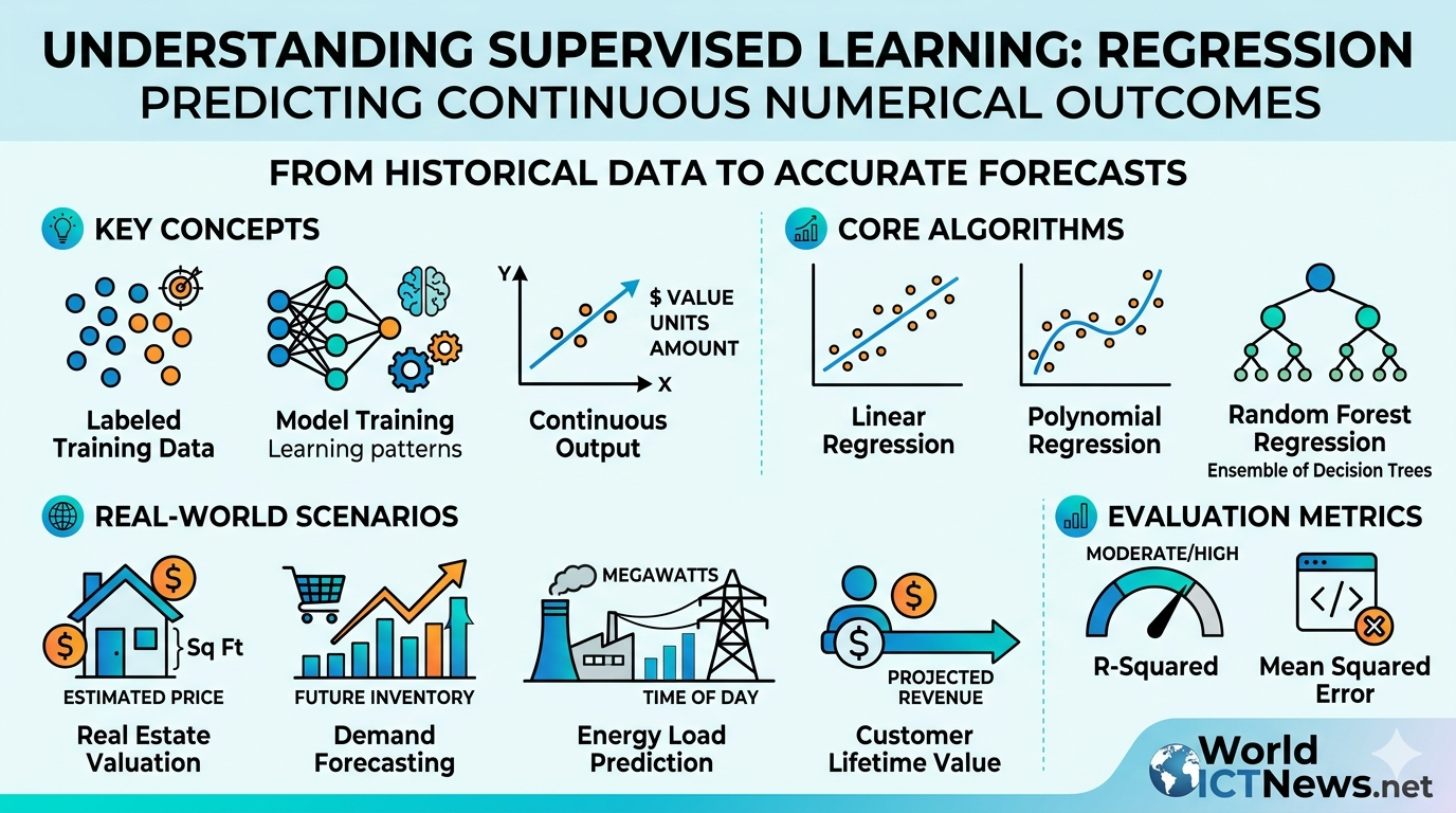
In a supervised learning ecosystem, a computer model learns historical patterns using labeled data. The model is supplied with a training dataset containing both independent variable characteristics (features) and the correct, historically verified output metrics (targets).

Mathematically, the core objective of a supervised regression algorithm is to approximate an underlying mapping function (\(f\)) that links an input vector (\(X\)) to a continuous, dependent output variable (\(Y\)):

\(Y=f(X)+\epsilon \)

Here, \(X\) represents the incoming feature data, \(Y\) is the numerical target value we want to predict, and \(\epsilon \) represents the irreducible random error or noise inherent to real-world environments.

During training, the model processes historical samples, calculates an initial prediction, checks its variance against the true target label using a mathematically defined loss function, and modifies its internal weights to reduce that error metric. This cycle loops until the model stabilizes. Once deployed, the system handles completely unlabelled, real-time feature variables and projects highly accurate numerical estimates.

2. Core Regression Algorithms

Depending on the distribution of data points and structural complexity, data scientists deploy several unique algorithmic architectures to fit a trendline:

Linear Regression

The most elementary yet robust form of regression analysis. Linear regression assumes a straight-line relationship exists between the input characteristics and the target variable.

• Simple Linear Regression: Maps a single input variable (\(x\)) to an output (\(y\)) using a straight line equation: \(y = \beta_0 + \beta_1x\).

• Multiple Linear Regression: Extends this concept to handle dozens of input metrics concurrently, defining a multidimensional plane of best fit: \(y = \beta_0 + \beta_1x_1 + \beta_2x_2 + \dots + \beta_nx_n\).

Polynomial Regression

When data points do not scale along a straight line, forcing a linear model onto them creates systemic errors. Polynomial regression solves this limitation by transforming the linear equation into a curved line model. It accomplishes this by squaring, cubing, or raising the input features to higher power degrees (e.g., \(y = \beta_0 + \beta_1x + \beta_2x^2\)), allowing the model to adapt smoothly to non-linear datasets.

Ridge and Lasso Regression (Regularization Techniques)

When models are trained on datasets containing too many competing features, they frequently over-respond to noise, making complex, erratic predictions. Ridge and Lasso regression prevent this by adding a mathematical penalty directly to the loss function:

• Ridge Regression (L2 Regularization): Forces feature weights closer to zero, smoothing out drastic variance spikes across the model.

• Lasso Regression (L1 Regularization): Can shrink unimportant feature weights all the way to absolute zero, acting as an automated feature selection tool that strips out useless data columns completely.

Decision Tree & Random Forest Regressors

Instead of relying on continuous algebraic formulas, Decision Trees slice datasets into increasingly smaller numerical zones based on strict conditional rules (e.g., Is age > 35?). A Random Forest Regressor combines an ensemble of hundreds of these individual trees, allowing each one to generate its own prediction. The final system output is calculated by taking the mathematical average of all the individual tree outputs, creating an incredibly resilient, non-linear forecasting tool.

3. Real-Life Scenarios and Applications

To understand how regression algorithms operate across modern business infrastructure, let us examine four real-world deployment scenarios.

Scenario A: Real Estate — Dynamic Property Valuation Matrix

• Regression Architecture: Multiple Linear Regression and Random Forest Regressors

• Primary Metrics Evaluated: Total Square Footage, Location Coordinates, Age of Structure, Historical Neighborhood Comp Sales

Property appraisal historically relied on manual local research, but digital real estate marketplaces now deploy automated valuation models (AVMs) to update millions of property evaluations in real-time.

[Input Features]                 [Regression Model]             [Continuous Output]
- 2,400 sq. ft.       -------\
- Zip Code: 90210     --------\   (Random Forest    -------->   Estimated Value:
- 4 Bedrooms / 3 Bath --------/     Regressor)                  $1,345,200.00
- Year Built: 2012    -------/

When a homeowner updates their listing information on an online platform, a regression pipeline pulls the property’s physical features and transforms them into numerical vectors. The model cross-references these vectors against recent surrounding transactions.

The baseline linear components calculate a standard price-per-square-foot valuation, while non-linear decision tree layers adjust the price down if the property sits directly adjacent to a noisy freeway, or scale it up if it falls within a top-tier school district. The system processes these attributes instantly to output a specific dollar valuation, giving buyers and sellers an immediate baseline market price.

Scenario B: E-Commerce & Retail — Predictive Supply Chain Demand Forecasting

• Regression Architecture: Polynomial Regression and Gradient Boosted Regressors

• Primary Metrics Evaluated: Historic Sales Volume, Promotional Ad Spend, Seasonal Temperature Adjustments, Competitor Pricing Indexes

Global retail platforms must anticipate consumer ordering patterns months in advance to prevent costly warehouse stockouts or bloated surplus inventories.

Consider an online apparel company planning its winter outerwear inventory. A regression model maps historic purchase orders alongside external seasonal vectors. The model recognizes that winter coat demand scales non-linearly: sales do not rise steadily as temperature drops; instead, sales spike exponentially the moment regional temperatures cross below the freezing point (32°F / 0°C).

By tracking these curves through polynomial and ensemble regression layers, the system models the incoming customer demand curve. If the algorithm forecasts an upcoming localized order volume of exactly 42,500 heavy winter parkas for the month of November, the logistics engine uses that continuous value to automate manufacturing queues and pre-ship inventory directly to regional fulfillment centers.

Scenario C: Energy Sector — Electrical Grid Load Projection

• Regression Architecture: Support Vector Regression (SVR) and Deep Learning Neural Regressors

• Primary Metrics Evaluated: Real-Time Smart Meter Consumption, Weather Forecast Data, Industrial Operation Schedules, Day of the Week

Electricity must be consumed the exact moment it is generated, as storing massive power overloads within grid networks remains highly inefficient. Power grid utility companies use regression algorithms to balance energy generation against ongoing consumer demand.

[System Inputs]                [Predictive Engine]              [Grid Output Layer]
- Temp: 98°F (Heatwave) ----\
- Day: Wednesday        -----\    (Support Vector   -------->   Required Output:
- Time: 4:00 PM         -----/      Regression)                 850 MegaWatts (MW)
- Industrial Activity   ----/

During a major summer heatwave, smart meters stream real-time consumption data back to utility operations. The regression model maps incoming atmospheric weather forecasts against historical baseline usage curves. The model identifies that at 4:00 PM on a working weekday during a 98°F heatwave, air conditioning units across a city will push energy consumption to a specific peak load—for example, exactly 850 MegaWatts.

By having access to this continuous numeric output ahead of time, grid engineers can ramp up auxiliary power plants or activate battery reserves precisely when needed, preventing blackouts while avoiding the financial waste of over-generating power.

Scenario D: Finance & Venture Capital — Customer Lifetime Value (CLV) Calculation

• Regression Architecture: Ridge Regression and Deep Neural Networks

• Primary Metrics Evaluated: Initial Purchase Value, App Engagement Metrics, Customer Acquisition Cost, Referral Tracking Counts

For subscription platforms and modern financial technologies to remain profitable, they must calculate exactly how much money a customer will spend over their entire relationship with the company.

When a user signs up for a digital streaming service or a trading app, their initial actions are tracked as feature metrics: how many videos they watch in the first week, how many custom playlists they build, and the value of their initial cash deposit.

A regularization regression model maps these usage habits against the lifespans of millions of past users. The system calculates a projected Customer Lifetime Value as a clear, continuous dollar amount (e.g., predicting user #40921 will generate exactly $248.50 in revenue over a 36-month period). Marketing departments use these regression values to dynamically adjust their digital advertising bids, ensuring they never spend more to acquire a new user than that user is mathematically projected to worth.

4. Technical Performance Evaluation

To verify that a regression model is making accurate numerical predictions rather than random guesses, data scientists track three core evaluation metrics:

• Mean Absolute Error (MAE): Measures the average absolute distance between the model's predictions and the actual target values. It tells us how far off our predictions are on average, expressed directly in the original unit of measurement (e.g., being off by an average of $5,000 on house prices).

• Mean Squared Error (MSE): Squares the error values before averaging them. Because it squares the distances, large errors are penalized heavily, making MSE an excellent tool for flagging models that make rare but catastrophic forecasting mistakes.

• R-Squared (\(R^{2}\) Score): Measures the proportion of variance in the dependent target variable that can be explained by the model's input features. An \(R^{2}\) score of 1.0 indicates a flawless model fit, while a score of 0.0 means the model performs no better than a simple average baseline.

5. Overview of Regression Use Cases

6. Practical Realities and Constraints

Building successful regression systems requires navigating several data anomalies that can disrupt performance:

Multi-Collinearity

This happens when two or more input features are highly correlated with each other (e.g., tracking both square footage and total room volume in a housing dataset). This overlap confuses linear models, making it difficult for the system to figure out which feature is actually driving the change in value. Data scientists use techniques like Lasso regression or Variance Inflation Factors (VIF) to clean up these redundant columns.

Sensitivity to Outliers

Simple regression models are highly sensitive to extreme data anomalies. For example, if you include a single billionaire's mansion in a dataset of modest suburban homes, a standard linear regression line will skew dramatically upward, ruining the model's accuracy for normal properties. Addressing this requires robust preprocessing, clipping extreme values, or swapping to outlier-resistant models like Huber Regression.

7. Summary

Supervised regression models provide a powerful framework for deciphering the continuous mathematical relationships that drive our physical and digital systems. By converting historical data trends into clear, actionable forecasting lines, regression helps organizations transition from reactive decision-making to highly precise predictive operations.