Probability Distribution Manual Calculation Procedures

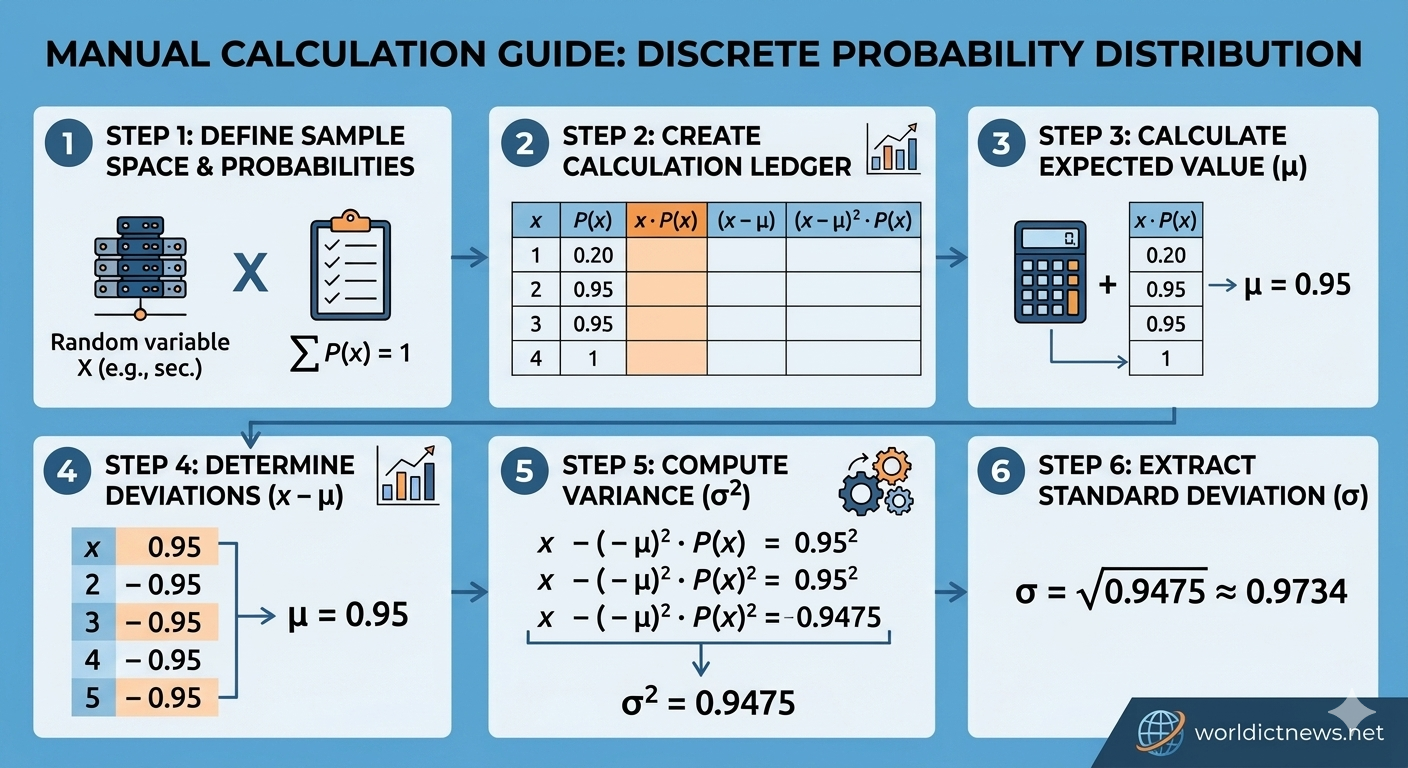
Step-by-Step Probability Distribution Manual Calculation.

In the fields of data science, machine learning, and statistical analysis, understanding how data points are distributed is foundational. While modern software pipelines and online calculators instantly compute statistical values, understanding the underlying mathematics is crucial for diagnosing modeling anomalies like data drift or skewed datasets.

A Probability Distribution is a mathematical function that describes the likelihood of obtaining the possible values that a random variable can take. This comprehensive, hands-on guide walks you through the step-by-step manual calculation of a discrete probability distribution. You will learn how to build a manual probability distribution table, calculate the expected value (mean), compute the variance, and determine the standard deviation without relying on external software tools.

1. Core Definitions: Random Variables and Distributions

To build a probability distribution calculator manually, you must first understand the type of data you are processing. Random variables are divided into two primary categories:

• Discrete Random Variables: Variables that take on a countable number of distinct values (e.g., the number of servers failing in a data center, or the number of support tickets received per hour).

• Continuous Random Variables: Variables that take on an infinite number of possible values within a continuous range (e.g., the execution time of a cloud function, or network latency in milliseconds).

This manual calculation guide focuses on Discrete Probability Distributions, which are governed by two mandatory mathematical axioms:

1. The probability of each individual outcome x must sit between 0 and 1 inclusive:
   0 <= P(X = x) <= 1

2. The sum of all individual probabilities across the entire sample space must equal exactly 1:
   Sum of P(x) = 1

2. Setting Up the Scenario Sample Space

Let us establish a practical IT infrastructure scenario to serve as our calculation baseline.

Suppose a DevOps engineering team tracks a cluster of 3 load balancers. Over a historical monitoring period, they record how many load balancers experience a localized configuration sync error during an automated deployment cycle.

The sample space for the number of affected load balancers (x) ranges from 0 to 3. Based on log frequency data, the underlying probability values are recorded as follows:

• Probability of 0 errors: 0.40

• Probability of 1 error: 0.35

• Probability of 2 errors: 0.15

• Probability of 3 errors: 0.10

Step 1: Verify the Distribution Axiom

Before executing advanced calculations, calculate the sum of your probabilities to verify the dataset is statistically valid:

Sum of P(x) = 0.40 + 0.35 + 0.15 + 0.10 = 1.00

The sum equals exactly 1.00, confirming the dataset is a valid probability distribution.

3. Constructing the Calculation Table

The most effective tool for manual distribution calculation is a multi-column matrix table. This structural layout breaks down complex formulas into simple arithmetic steps, reducing calculation errors.

Create a blank ledger containing five core columns:

1. x: The individual random variable outcomes.

2. P(x): The corresponding probability of each outcome.

3. x * P(x): The product used to calculate the Expected Value.

4. (x - Mean): The deviation of each outcome from the calculated mean.

5. (x - Mean)^2 * P(x): The weighted squared deviation used to calculate Variance.

Let's populate the primary inputs:

4. Step-by-Step Calculation of Expected Value (Mean)

The Expected Value, mathematically denoted as E(X) or the symbol Mean, represents the long-term average outcome if the random event were repeated an infinite number of times.

The formula for the expected value of a discrete distribution is:
Mean = Sum of [x * P(x)]

Step 2: Calculate the product for each row

• Row 1 (x=0): 0 * 0.40 = 0.00

• Row 3 (x=1): 1 * 0.35 = 0.35

• Row 3 (x=2): 2 * 0.15 = 0.30

• Row 4 (x=3): 3 * 0.10 = 0.30

Step 3: Sum the products

Add the values together to find the expected value (Mean):

Mean = 0.00 + 0.35 + 0.30 + 0.30 = 0.95

Statistical Interpretation: If the engineering team runs thousands of deployments, they can expect an average of 0.95 errors per deployment cycle.

5. Step-by-Step Calculation of Variance

The Variance, denoted as Variance or Var(X), measures the dispersion of the distribution. It quantifies how far the individual outcomes spread out from the expected value (Mean = 0.95) we just calculated.

The formula for calculating variance manually is:
Variance = Sum of [(x - Mean)^2 * P(x)]

Step 4: Calculate the deviation column (x - Mean)

Subtract the mean (0.95) from each individual outcome (x):

• Row 1 (x=0): 0 - 0.95 = -0.95

• Row 2 (x=1): 1 - 0.95 = 0.05

• Row 3 (x=2): 2 - 0.95 = 1.05

• Row 4 (x=3): 3 - 0.95 = 2.05

Step 5: Square the deviations and multiply by P(x)

Square each deviation result to eliminate negative signs, then multiply that result by the row's corresponding probability:

• Row 1 (x=0): (-0.95)^2 0.40 = 0.9025 0.40 = 0.3610

• Row 2 (x=1): (0.05)^2 0.35 = 0.0025 0.35 = 0.000875

• Row 3 (x=2): (1.05)^2 0.15 = 1.1025 0.15 = 0.165375

• Row 4 (x=3): (2.05)^2 0.10 = 4.2025 0.10 = 0.42025

Step 6: Sum the weighted squared deviations

Add the values from the final column to find the total variance:

Variance = 0.3610 + 0.000875 + 0.165375 + 0.42025 = 0.9475

6. Step-by-Step Calculation of Standard Deviation

While variance is mathematically valuable, its units are squared (e.g., "0.9475 errors squared"), making it difficult to interpret alongside raw data. To return to our baseline unit of measurement, we calculate the Standard Deviation.

The standard deviation is simply the positive square root of the variance:
Standard Deviation = Square Root of (Variance)

Step 7: Extract the square root

Using a standard manual calculations block for the Square Root of 0.9475:

Standard Deviation = Square Root of (0.9475) = 0.9734

Final Analysis Profile: Our calculated system profile shows an expected error rate of 0.95 errors with a standard deviation of 0.9734 errors. This indicates a high level of variability relative to the mean, signaling that error rates fluctuate significantly between different deployment cycles.

7. The Completed Reference Ledger Table

Below is the fully calculated distribution table. This serves as the reference blueprint for verifying manual arithmetic:

Conclusion

Building a probability distribution calculator manually requires a methodical, step-by-step approach to processing outcomes, probabilities, and statistical averages. By validating the baseline axioms, constructing a ledger table, and processing expected values, variance, and standard deviation sequentially, you can calculate discrete distributions accurately without software dependencies. This core mathematical workflow forms the foundation for data modeling, risk profiling, and complex algorithmic processing across tech and data sectors.

Frequently Asked Questions (FAQ)

1. What happens if the sum of my P(x) column does not equal 1?

If the sum of your probabilities does not equal exactly 1.0, your dataset is structurally invalid or incomplete. Double-check your initial log figures for math errors, or ensure that you have accounted for every possible outcome in your sample space.

2. Can an individual deviation value (x - Mean) be negative?

Yes, individual deviation values will be negative whenever an outcome (x) is smaller than the calculated distribution mean. However, these negative values disappear in the next step when you square the deviations.

3. What is the alternative formula for calculating variance manually?

An alternative formula for variance is the computational formula: Variance = Sum of [x^2 * P(x)] - Mean^2. This method skips the individual deviation column by summing the products of the squared outcomes and probabilities, then subtracting the squared mean at the very end.

4. What does a standard deviation close to 0 indicate?

A standard deviation close to 0 indicates that the random variable outcomes are tightly clustered around the expected value, signaling high predictability and low variance across cycles.

5. Is this manual calculation method applicable to continuous variables?

No, this specific tabular summation method applies only to discrete random variables. Continuous random variables require integral calculus over a specific probability density function (PDF) boundary to find mean and variance.