The Architecture of Cluster Analysis: Mathematical Frameworks and Algorithmic Blueprints

The Architecture of Cluster Analysis: Mathematical Frameworks, Algorithmic Blueprints, and Production Python Architectures.

In the era of big data, organizations ingest massive volumes of unlabelled, multi-dimensional information every second. Whether processing high-frequency e-commerce transaction logs, streaming multi-spectral satellite telemetry, or managing clinical patient biometric profiles, data scientists face a common hurdle: finding meaningful, hidden structures in data without pre-existing training labels.

Traditional machine learning relies heavily on supervised paradigms like classification and regression. However, supervised models are fundamentally helpless when a business does not possess historical target outcomes or categories. To uncover the organic taxonomies, underlying customer personas, or anomaly vectors buried within unlabelled datasets, we must deploy Cluster Analysis.

Cluster analysis (or clustering) is the unsupervised task of grouping a set of data objects into distinct partitions. The structural goal is straightforward: maximize intra-cluster similarity (objects inside the same cluster should be as close to one another as possible) while maximizing inter-cluster disparity (separate clusters should be as distinct and distant from one another as possible).

This comprehensive masterclass breaks down the foundational math of distance spaces, analyzes three major algorithmic paradigms (Centroid-based, Density-based, and Hierarchical), evaluates clustering quality using rigorous verification metrics, and provides a production-grade Python workflow with real-world business case studies.

1. The Mathematical Core: Proximity Measures and Distance Spaces

At the center of every clustering algorithm sits a proximity metric. Because unsupervised models lack historical outcome labels to judge correctness, they rely on geometric distance calculations to define what makes two observations "similar."

The selection of a distance space determines the geometric shape of the resulting clusters. If you change the metric, you alter how the algorithm maps boundaries across the feature grid.

                  ┌──────────────────────────────┐
                  │      Distance Spaces         │
                  └──────────────┬───────────────┘
                                 │
         ┌───────────────────────┼───────────────────────┐
         ▼                       ▼                       ▼
    [ Euclidean ]          [ Manhattan ]          [ Cosine Space ]
  Straight-Line (L2)       Grid-Based (L1)       Directional Angle

Euclidean Distance (L2 Norm)

The most common geometric metric used in data science is Euclidean Distance. It calculates the straight-line distance between two coordinates in a multi-dimensional Cartesian space.

• Plain-Text Formula: For two n-dimensional observations, P = (p1, p2, ... pn) and Q = (q1, q2, ... qn), the Euclidean distance is defined as:

Distance(P, Q) = sqrt( sum( (pi - qi)^2 ) )

• Operational Caveat: Euclidean space assumes all features are continuous, normally distributed, and scaled equally. If one feature represents annual revenue in millions and another represents customer age in years, the revenue variable will completely overwhelm the calculation. Therefore, standardizing features via Z-score normalization or Min-Max scaling is a mandatory pre-requisite before applying Euclidean-based models.

Manhattan Distance (L1 Norm / Taxicab Geometry)

Instead of cutting diagonally across coordinates, Manhattan Distance measures the path along axes at right angles.

• Plain-Text Formula:

Distance(P, Q) = sum( abs( pi - qi ) )

• Operational Fit: Manhattan distance is highly robust when analyzing datasets with high dimensionality. As the number of dimensions scales upward, Euclidean distances tend to become uniform (a phenomenon known as the curse of dimensionality). The L1 norm helps preserve contrast between data points in dense feature environments.

Cosine Similarity & Distance

When the absolute magnitude of features matters less than the relative direction or orientation of the data vectors, we shift to Cosine Space. This is standard in text mining, natural language processing (NLP), and user recommendation systems.

• Plain-Text Formula: It calculates the cosine of the angle theta between two multi-dimensional vectors:

Similarity(P, Q) = cos(theta) = (P dot Q) / (norm(P) * norm(Q))

Cosine Distance = 1 - Similarity(P, Q)

• Operational Fit: If you are clustering documents based on word frequencies, a short 100-word article and a massive 10,000-word essay might cover the exact same topic. Euclidean distance will mark them as incredibly far apart due to total word counts. Cosine distance looks strictly at the vector angle, correctly clustering them together based on proportional keyword alignment.

2. Core Algorithmic Frameworks

No single clustering algorithm fits every dataset. Data structures vary: some consist of neat, spherical groups, while others form winding, intertwined density paths. Data scientists choose models from three major structural families.

Family A: Centroid-Based Models (K-Means)

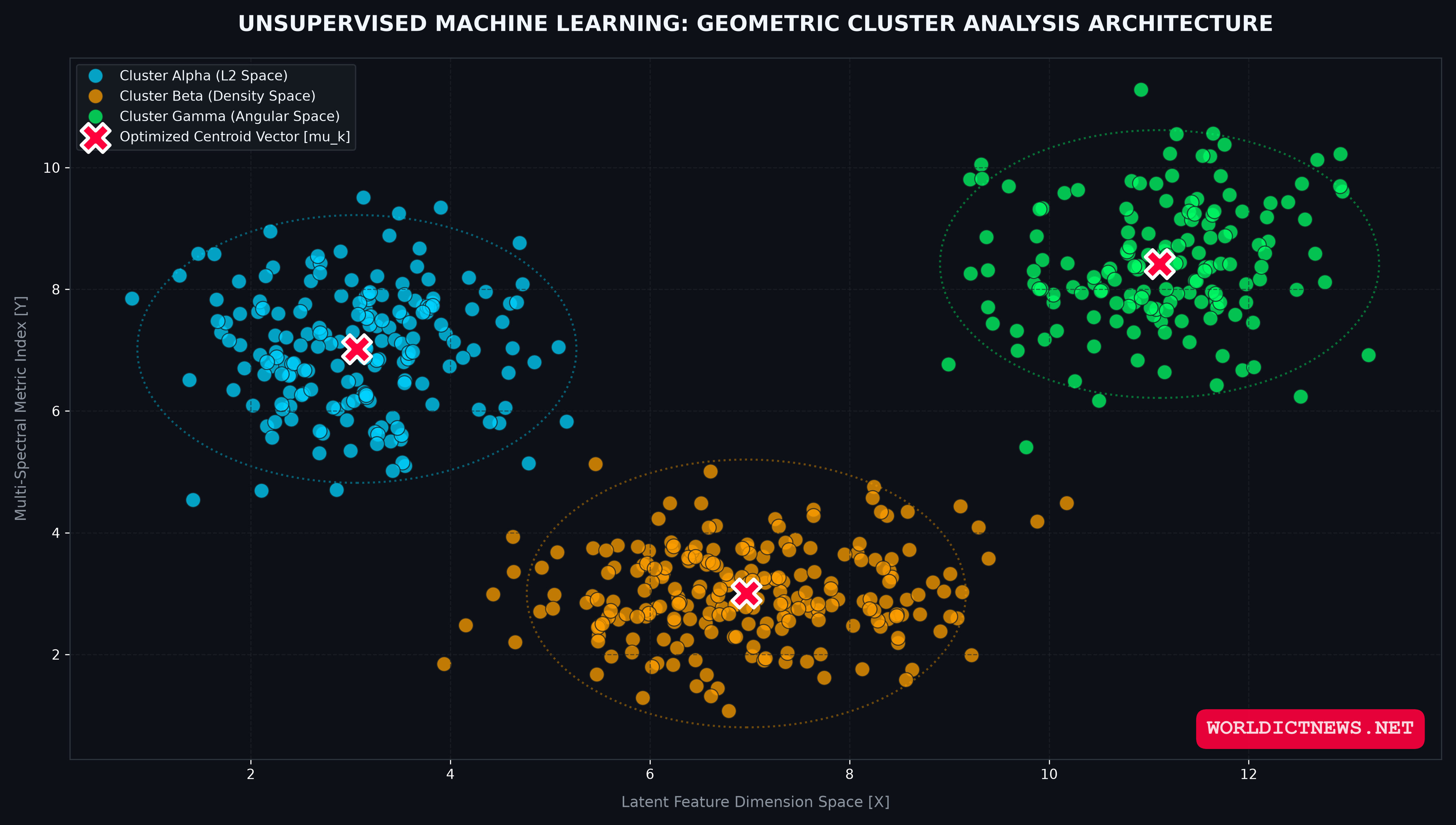
K-Means is the workhorse of unsupervised learning. It aims to partition N observations into K distinct clusters, where each observation belongs to the cluster with the nearest mean (centroid).

  [ Initial Random Centroids ] ──► [ Assign Points to Nearest Mean ] ──┐
                ▲                                                      │
                └─────────────── [ Recalculate Centroid Means ] ───────┘

The model iteratively optimizes the Within-Cluster Sum of Squares (WCSS), also known as Inertia:

WCSS = sum_k( sum_xi_in_Ck( norm( xi - mu_k )^2 ) )

Where Ck is the set of points in cluster k, and mu_k is the calculated mean centroid of that cluster.

The Operational Lifecycle of K-Means:

1. Initialization: The user specifies the exact number of clusters (K). The algorithm places K random starting centroids across the feature grid (often using the advanced k-means++ initialization routine to spread them out efficiently).

2. Assignment Step: Every observation in the dataset is assigned to its closest starting centroid based on Euclidean distance.

3. Update Step: The algorithm calculates the geometric mean of all coordinates assigned to each cluster, moving the centroids to these new center points.

4. Convergence: The Assignment and Update phases loop continuously until the centroids stop shifting or the maximum iteration threshold is hit.

• Structural Weakness: K-Means assumes clusters are spherical, roughly equal in size, and have similar density spreads. It fails completely when confronted with complex geometric patterns, elongated configurations, or heavy background noise.

Family B: Density-Based Models (DBSCAN)

DBSCAN (Density-Based Spatial Clustering of Applications with Noise) approaches data by grouping points based on spatial concentration rather than center points.

Unlike K-Means, DBSCAN does not force you to guess the number of clusters in advance. It identifies clusters of arbitrary shapes and automatically flags isolated data points as background noise.

Core Structural Parameters:

• Epsilon (Eps): The maximum radius distance to search for neighboring points around a coordinate.

• MinSamples: The minimum number of points required within the Epsilon radius to declare that area a dense region.

The Classification of Data Points:

• Core Points: Any coordinate that contains at least the MinSamples count inside its Epsilon neighborhood.

• Border Points: Points that do not have enough neighbors to be core points, but fall inside the Epsilon radius of a valid Core Point.

• Noise Points (Outliers): Any observation that is neither a Core Point nor a Border Point. These are ignored by clusters, making DBSCAN highly resilient to anomalies.

      (  Core Point  )  ──► [ High neighbor density within Epsilon ]
     (  Border Point  ) ──► [ Low neighbor density, but touches a Core Point ]
    [   Noise Point   ] ──► [ Isolated outlier; excluded from all clusters ]

• Structural Weakness: DBSCAN struggles when analyzing datasets with highly variable densities. If one cluster is tightly packed and another is loosely spread, a single Epsilon value cannot capture both boundaries cleanly.

Family C: Hierarchical Models (Agglomerative)

Agglomerative Hierarchical Clustering builds a tree of clusters using a bottom-up methodology.

The Assembly Pipeline:

1. Every observation starts as its own individual single-point cluster (N items = N clusters).

2. The algorithm calculates the distance between all clusters and merges the two closest ones into a joint group.

3. The merging loops continuously until all observations are unified into a single root cluster.

Linkage Matrix Criteria:

To determine the distance between clusters containing multiple points, developers choose specific linkage parameters:

• Ward Linkage: Minimizes the total variance increment within clusters during merges. This yields highly spherical, balanced clusters.

• Complete Linkage: Computes the distance between the two furthest points across clusters.

• Single Linkage: Computes the distance between the two closest points across clusters. This is prone to chaining effects, where trailing noise points accidentally bridge distinct clusters together.

The entire hierarchical structural tree is visualized using a graphic called a Dendrogram. This allows practitioners to visually cut across branches to choose the optimal number of clusters after the processing phase completes.

3. High-Value Business Case Study: Customer Segmentation Workflow in Python

💼 Business Context

An international e-commerce platform wants to optimize its seasonal marketing campaigns. Rather than blasting millions of generic promotional emails to their entire user base, they want to isolate distinct customer purchasing personas based on transaction values, website interaction metrics, and loyalty patterns.

🎯 Objective

Simulate a production-level dataset of 500 customers, execute data preprocessing, determine the optimal cluster configuration using diagnostic indices, deploy an optimized K-Means engine, and output high-resolution visualization profiles.

🛠️ Production Verification Command

To execute this analytical workflow natively inside Visual Studio Code, ensure your system terminal has the required data science library suite installed:

bash

pip install numpy pandas matplotlib seaborn scikit-learn

Use code with caution.

Python Blueprint Implementation (customer_segmentation.py)

python

import numpy as np
import pandas as pd
import matplotlib.pyplot as plt
import seaborn as sns
from sklearn.preprocessing import StandardScaler
from sklearn.cluster import KMeans
from sklearn.metrics import silhouette_score, calinski_harabasz_score

# ==========================================
# 1. GENERATE SYNTHETIC CUSTOMER TRANS_LOGS
# ==========================================
np.random.seed(42)

# Generate three distinct target populations (Personas)
# Group 1: High Spending, Low Engagement (VIP Bargainers)
g1_spend = np.random.normal(loc=120, scale=15, size=150)
g1_engage = np.random.normal(loc=30, scale=5, size=150)

# Group 2: Low Spending, High Engagement (Loyal Browsers)
g2_spend = np.random.normal(loc=40, scale=10, size=200)
g2_engage = np.random.normal(loc=85, scale=8, size=200)

# Group 3: High Spending, High Engagement (Core Brand Champions)
g3_spend = np.random.normal(loc=200, scale=25, size=150)
g3_engage = np.random.normal(loc=75, scale=10, size=150)

# Unified Data Frames Assembly
df_spend = np.concatenate([g1_spend, g2_spend, g3_spend])
df_engage = np.concatenate([g1_engage, g2_engage, g3_engage])

df_customers = pd.DataFrame({
    'Annual_Spend_USD': df_spend,
    'Engagement_Score': df_engage
})

print("--- RAW CUSTOMER TRANSACTION LOG METRICS ---")
print(df_customers.head())
print(f"Total Customer Datasets: {df_customers.shape} Rows\n")

# ==========================================
# 2. DATA PREPROCESSING & STANDARDIZATION
# ==========================================
# Standardize features to have a mean of 0 and variance of 1
scaler = StandardScaler()
scaled_features = scaler.fit_transform(df_customers)

# ==========================================
# 3. DIAGNOSTIC SCANS: TARGET SELECTION
# ==========================================
wcss_inertia = []
silhouette_coefficients = []
k_range = range(2, 11)

for k in k_range:
    kmeans_eval = KMeans(n_clusters=k, init='k-means++', random_state=42, n_init=10)
    kmeans_eval.fit(scaled_features)
    
    wcss_inertia.append(kmeans_eval.inertia_)
    silhouette_coefficients.append(silhouette_score(scaled_features, kmeans_eval.labels_))

# Plot Diagnostic Curves (Elbow and Silhouette)
fig, (ax1, ax2) = plt.subplots(1, 2, figsize=(16, 5))

# Elbow Method Plot
ax1.plot(k_range, wcss_inertia, marker='o', color='#1A365D', linewidth=2)
ax1.set_title('Elbow Validation Diagnostic: Minimizing WCSS', fontsize=11, fontweight='bold', color='#1A365D')
ax1.set_xlabel('Cluster Count (K)')
ax1.set_ylabel('Within-Cluster Sum of Squares (Inertia)')
ax1.grid(True, linestyle='--', alpha=0.5)

# Silhouette Analysis Plot
ax2.plot(k_range, silhouette_coefficients, marker='s', color='#2B6CB0', linewidth=2)
ax2.set_title('Silhouette Framework Scan: Maximizing Separation Coeff', fontsize=11, fontweight='bold', color='#2C5282')
ax2.set_xlabel('Cluster Count (K)')
ax2.set_ylabel('Average Silhouette Coefficient')
ax2.grid(True, linestyle='--', alpha=0.5)

plt.tight_layout()
plt.savefig("clustering_diagnostics.png", dpi=300)
print("DIAGNOSTIC VISUALIZATION LOGGED: 'clustering_diagnostics.png' saved to disk.")

# ==========================================
# 4. OPTIMIZED ENGINE DEPLOYMENT (K=3 chosen)
# ==========================================
optimal_k = 3
final_engine = KMeans(n_clusters=optimal_k, init='k-means++', random_state=42, n_init=10)
cluster_assignments = final_engine.fit_transform(scaled_features)
df_customers['Cluster_ID'] = final_engine.labels_

# ==========================================
# 5. METRIC QUANTIFICATION MATRIX
# ==========================================
sil_avg = silhouette_score(scaled_features, final_engine.labels_)
ch_score = calinski_harabasz_score(scaled_features, final_engine.labels_)

print("\n=== SYSTEM PERFORMANCE EVALUATION METRICS ===")
print(f"Final Configured Clusters (K): {optimal_k}")
print(f"Average Silhouette Score: {sil_avg:.4f}")
print(f"Calinski-Harabasz Variance Score: {ch_score:.2f}\n")

# ==========================================
# 6. PRODUCTION SUMMARY CLUSTER SEGMENTS
# ==========================================
cluster_profile_summary = df_customers.groupby('Cluster_ID').mean()
print("=== CLUSTER PROFILED MEAN SEGMENTATION SUMMARIES ===")
print(cluster_profile_summary)

# ==========================================
# 7. HIGH-RESOLUTION EXPEDITION GRAPH
# ==========================================
plt.figure(figsize=(12, 8))
sns.scatterplot(
    data=df_customers, 
    x='Annual_Spend_USD', 
    y='Engagement_Score', 
    hue='Cluster_ID', 
    palette=['#1A365D', '#DD6B20', '#2F855A'],
    s=100, 
    alpha=0.8,
    edgecolor='w'
)

# Convert Centroids back to original unscaled feature parameters for plotting
unscaled_centroids = scaler.inverse_transform(final_engine.cluster_centers_)
plt.scatter(
    unscaled_centroids[:, 0], 
    unscaled_centroids[:, 1], 
    s=350, 
    color='red', 
    marker='X', 
    edgecolor='black', 
    linewidth=2,
    label='Optimized Cluster Centroids'
)

plt.title('Systems Analytics Workspace: Corporate Customer Segmentation Engine', fontsize=13, fontweight='bold', color='#1A365D')
plt.xlabel('Annual Customer Spend Architecture (USD / Year)')
plt.ylabel('Digital Interface Engagement Index Score (0 - 100)')
plt.grid(True, linestyle=':', alpha=0.6)
plt.legend(loc='upper right')

plt.savefig("customer_segmentation_output.png", dpi=300)
print("PRODUCTION METRIC MAP EXPORT SUCCESS: 'customer_segmentation_output.png' saved.")
plt.show()

Use code with caution.

4. Mathematical Validation Frameworks: Interpreting the Scores

Because cluster analysis does not check its outputs against predefined ground-truth labels, models can easily group random noise into arbitrary clusters. To ensure our generated clusters represent real physical boundaries rather than statistical alignment artifacts, we rely on two key validation frameworks:

1. The Silhouette Coefficient

The Silhouette Score measures how clean the geometric separation between clusters is. For an individual observation i, its silhouette coefficient s(i) is defined as:

s(i) = ( b(i) - a(i) ) / max( a(i), b(i) )

Where:

• a(i) is the mean intra-cluster distance between point i and all other coordinates in the same cluster. It maps compactness.

• b(i) is the mean nearest-cluster distance between point i and all points in the closest neighboring cluster. It maps separation.

Interpretation Matrix:

• Near +1.0 Score: Points are located far away from parallel clusters, indicating a clean, highly resilient structural partition.

• Near 0.0 Score: The coordinate sits directly on the boundary line between two overlapping clusters, signaling high system ambiguity.

• Negative Score: The observation has been grouped into the wrong cluster entirely.

2. The Calinski-Harabasz Index (Variance Ratio Criterion)

The Calinski-Harabasz score computes the ratio of the sum of between-clusters variance to the within-cluster variance.

CH Score = ( SSB / SSW ) * ( (N - K) / (K - 1) )

Where SSB is the variance between different clusters, SSW is the variance inside individual clusters, N is the total number of observations, and K is the number of clusters.

• The Logic: A higher Calinski-Harabasz score indicates that the clusters are both tightly packed internally and spaced widely apart externally, making it an excellent diagnostic metric for choosing the optimal cluster count.

5. Comparative Diagnostics Summary Matrix

To choose the optimal model layout across diverse feature environments, reference this baseline algorithm selection guide:

6. Operational Best Practices for Production Deployment

• Always Apply Feature Scaling: If your inputs use mismatched dimensions (e.g., matching a binary 0/1 gender flag against a $100,000 income column), distance-based models will focus entirely on the larger metric range. Apply Z-score standardization (StandardScaler) to give all features an equal footing.

• Mind the Curse of Dimensionality: As you add more variables to a dataset, the geometric volume of the space expands rapidly. This causes distances between points to become uniformly wide, making Euclidean metrics less effective. Use dimensionality reduction techniques like PCA (Principal Component Analysis) or t-SNE to compress your features down to core components before running your clustering models.

• Avoid Over-interpreting Inertia Curves: When running the K-Means Elbow method, the WCSS line will drop naturally every time you increase the cluster count (K), hitting zero when K equals the number of data points. Look for a clear, sharp bend in the curve where adding more clusters yields diminishing returns, and verify this point against your average Silhouette score.

• Establish Baseline Reproducibility: Because algorithms like K-Means pick random initial coordinates for their starting centroids, running the same script twice can yield slightly different results. Always fix your execution pipeline by setting a constant seed parameter (e.g., random_state=42) to guarantee your results are reproducible across production environments.