The Definitive Guide to T-Test Calculations Using PSPP

The Definitive Guide to T-Test Calculations Using PSPP: Theory, Procedures, and Practical Examples.

Introduction

In quantitative research, comparing the mean scores of different groups or conditions is a fundamental task. Researchers often need to determine if an observed difference between two averages is statistically meaningful or simply a result of random sampling variation. To answer this question, analysts rely on the T-Test, a family of parametric statistical tests developed by William Sealy Gosset under the pseudonym "Student."

While commercial statistical software suites like IBM SPSS are widely used for these calculations, their prohibitive licensing costs present significant barriers for independent researchers, students, and institutions in developing regions. PSPP serves as a powerful, free, open-source alternative. It mirrors the user interface, functionalities, and syntax language of SPSS, allowing users to execute complex statistical analyses seamlessly.

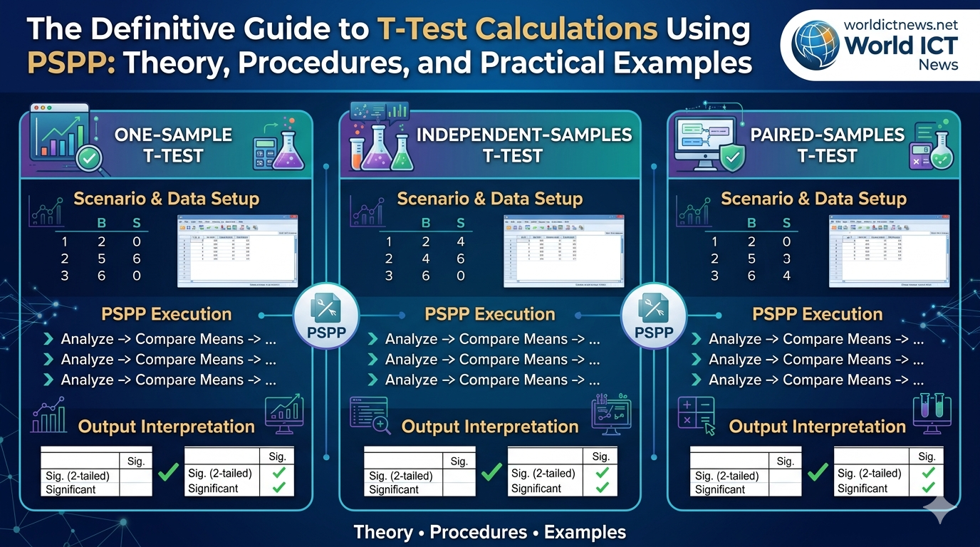
This comprehensive guide provides step-by-step procedures for calculating the three primary types of T-Tests using PSPP: One-Sample T-Tests, Independent-Samples T-Tests, and Paired-Samples (Dependent) T-Tests. Each procedure is accompanied by a practical research scenario, a concrete example dataset, step-by-step data configuration instructions, and a framework for output interpretation.

1. Fundamentals of the T-Test Family

Before executing commands in PSPP, it is vital to understand which T-Test fits your research design. All T-Tests compare means, but they differ based on where the data originates.

The Three Varieties of T-Tests

• One-Sample T-Test: Compares the mean of a single sample against a known or predetermined population mean or hypothetical test value.

• Independent-Samples T-Test: Compares the means of two distinct, unrelated groups (e.g., males vs. females, treatment group vs. control group) on the same continuous variable.

• Paired-Samples T-Test (Dependent T-Test): Compares the means of the same group of subjects at two different points in time or under two different conditions (e.g., pre-test vs. post-test scores).

Core Statistical Assumptions

To ensure the mathematical validity of your T-Test results in PSPP, your dataset should satisfy the following parameters:

1. Continuous Scale: The dependent variable must be measured at the interval or ratio level.

2. Independence of Observations: There must be no relationship between the observations within each group (crucial for Independent T-Tests).

3. Normal Distribution: The dependent variable should be approximately normally distributed within each group.

4. Homogeneity of Variance: For independent designs, the variances of the two groups should be roughly equal (tested via Levene's Test in PSPP).

2. Procedure 1: One-Sample T-Test

Scenario & Example Dataset

A university claims that its graduating seniors spend an average of 15 hours per week studying outside of class. A student researcher suspects the actual study time is different. They collect data from 8 randomly selected seniors.

• Hypothetical Population Mean (Test Value): 15

• Sample Data (Hours per week): 12, 14, 18, 11, 13, 16, 12, 10

Data Entry in PSPP

1. Launch PSPP and select the Variable View tab at the bottom left.

2. In row 1, type Study_Hours under the Name column. Set Decimals to 0 and type Weekly Study Hours under Label.

3. Switch to the Data View tab.

4. In the Study_Hours column, enter the 8 data points vertically into rows 1 through 8.

Study_Hours
-----------
12
14
18
11
13
16
12
10

Execution Steps

1. Navigate to the top menu bar and select Analyze \(\rightarrow \) Compare Means \(\rightarrow \) One Sample T Test...

2. A dialog box will open. Select Weekly Study Hours [Study_Hours] from the left panel and click the arrow button (\(\rightarrow \)) to move it into the Test Variable(s) window.

3. Locate the field labeled Test Value at the bottom of the box. Delete the default 0 and type 15.

4. Click OK.

Output Interpretation

PSPP will display two tables in the Output Viewer: "One-Sample Statistics" and "One-Sample Test".

One-Sample Statistics
============
Variable | N | Mean | Std. Deviation | SE. Mean
----+-----+----+----+-----
Weekly Study Hours | 8 | 13.25 | 2.60 | 0.92
=============

One-Sample Test
==============
Test Value = 15
----------------

| | | | Mean | 95% Conf. Int.
Variable | t | df | Sig. | Difference | Lower | Upper
---+--+--+---+----+--+---
Weekly Study Hours | -1.90| 7 | 0.100 | -1.75 | -3.92 | 0.42
=============

• Mean: The sample mean is 13.25 hours, which is lower than the claimed 15 hours.

• t-value: The calculated test statistic is -1.90.

• df (Degrees of Freedom): Calculated as \(N - 1 = 7\).

• Sig. (2-tailed): This is your p-value, which is 0.100.

• Statistical Decision: Because the p-value (\(0.100\)) is greater than the standard significance threshold (\(\alpha = 0.05\)), you fail to reject the null hypothesis. The difference between the sample mean (13.25) and the claimed mean (15) is not statistically significant.

3. Procedure 2: Independent-Samples T-Test

Scenario & Example Dataset

An instructional designer wants to evaluate if a new interactive e-learning platform results in higher exam scores compared to traditional textbook learning. They test two independent groups of students.

• Group 1 (Textbook): 5 students

• Group 2 (E-Learning): 5 students

• Dependent Variable: Test Score (out of 100)

Data Entry in PSPP

Unlike spreadsheets where groups are placed side-by-side, statistical packages require a Grouping Variable (categorical code) and a Test Variable (continuous data).

1. In Variable View, define two variables:

   • Row 1: Name = Method, Type = Numeric, Decimals = 0, Label = Instructional Method.

   • Row 2: Name = Score, Type = Numeric, Decimals = 0, Label = Exam Score.

2. Click on the Value Labels cell for the Method variable. Define the groups:

   • Value: 1 \(\rightarrow \) Label: Textbook \(\rightarrow \) Click Add.

   • Value: 2 \(\rightarrow \) Label: E-Learning \(\rightarrow \) Click Add \(\rightarrow \) Click OK.

3. Switch to Data View and arrange the 10 cases vertically:

Method | Score
-------+-------
  1    |   75
  1    |   82
  1    |   78
  1    |   70
  1    |   80
  2    |   85
  2    |   89
  2    |   94
  2    |   80
  2    |   88

Execution Steps

1. Select Analyze \(\rightarrow \) Compare Means \(\rightarrow \) Independent-Samples T Test...

2. Move Exam Score [Score] into the Test Variable(s) window.

3. Move Instructional Method [Method] into the Grouping Variable box.

4. Notice that the Define Groups button becomes clickable. Click it.

5. Type 1 into Group 1 and 2 into Group 2. Click Continue.

6. Click OK.

Output Interpretation

The Output Viewer yields a group breakdown and a comprehensive split test matrix.

Group Statistics
=========
Method | N | Mean | Std. Deviation | SE. Mean
--+-+--+--+-----
Textbook | 5 | 77.00 | 4.64 | 2.07
E-Learning | 5 | 87.20 | 5.12 | 2.29
==========

Independent Samples Test
=========
Levene's Test for Equality of Variances: F = 0.081 | Sig. = 0.784
-------------

| t | df | Sig.(2-tail) | Mean Difference
--+--+--+-+---
Equal var. assumed | -3.31 | 8 | 0.011 | -10.20
Equal var. not assumed| -3.31 | 7.92 | 0.011 | -10.20
==========

• Step 1: Check Levene's Test. Look at Sig. = 0.784. Because this value is much greater than \(0.05\), the variances are equal. We read the data from the row labeled Equal variances assumed.

• t-value and df: \(t = -3.31\) with \(8\) degrees of freedom.

• Sig. (2-tailed): The p-value is 0.011.

• Statistical Decision: Since \(0.011 < 0.05\), the result is statistically significant. The E-Learning group achieved a significantly higher mean test score (\(87.20\)) compared to the Textbook group (\(77.00\)).

4. Procedure 3: Paired-Samples T-Test

Scenario & Example Dataset

A medical clinic evaluates a new 4-week exercise regimen designed to reduce systolic blood pressure. The researcher records the blood pressure of 6 participants before starting the program and immediately after completion.

Data Entry in PSPP

Because the samples are paired (dependent), each row must represent an individual subject with both measurements placed side-by-side.

1. In Variable View, define two variables:

   • Row 1: Name = Pre_BP, Label = Systolic BP Before

   • Row 2: Name = Post_BP, Label = Systolic BP After

2. Switch to Data View and enter the data across 6 rows:

Pre_BP | Post_BP
-------+--------
  145  |   138
  138  |   132
  150  |   142
  160  |   151
  135  |   136
  142  |   139

Execution Steps

1. Navigate to Analyze \(\rightarrow \) Compare Means \(\rightarrow \) Paired-Samples T Test...

2. Click on Systolic BP Before [Pre_BP] and then click on Systolic BP After [Post_BP].

3. Click the arrow button (\(\rightarrow \)) to move the selected combination into the Paired Variables window as a linked pair (Pre_BP - Post_BP).

4. Click OK.

Output Interpretation

Paired Samples Statistics
=========
Variable | N | Mean | Std. Deviation | SE. Mean
---+-+--+--+---
Systolic BP Before | 6 | 145.33 | 8.78 | 3.58
Systolic BP After | 6 | 139.67 | 6.47 | 2.64
==========

Paired Samples Test
=========

| | | | Mean | 95% Conf. Int.
Pair 1 | t | df | Sig.2 | Diff. | Lower | Upper
-+-+-+-+--+--+--
Pre_BP - Post_BP | 4.11 | 5 | 0.009 | 5.67 | 2.12 | 9.21
==========

• Means Comparison: The mean blood pressure dropped from 145.33 mmHg before the program to 139.67 mmHg after.

• Mean Difference: The average net reduction per person was 5.67 mmHg.

• t-value and df: \(t = 4.11\) with \(5\) degrees of freedom.

• Sig. (2-tailed): The p-value is 0.009.

• Statistical Decision: Since \(0.009 < 0.05\), the drop in blood pressure is statistically significant. The 4-week exercise program is an effective intervention for lowering systolic blood pressure.

5. Alternative Execution: Using PSPP Syntax Workspace

If you want to bypass the graphical user interface or run your data analysis via scripting for reproducibility, you can use PSPP Syntax.

1. Open a new window by choosing File \(\rightarrow \) New \(\rightarrow \) Syntax.

2. Depending on your chosen analysis, paste one of the following code blocks:

spss

* --- COMMAND FOR ONE-SAMPLE T-TEST ---
T-TEST
/TESTVAL=15
/VARIABLES=Study_Hours.

* --- COMMAND FOR INDEPENDENT-SAMPLE T-TEST ---
T-TEST
/GROUPS=Method(1, 2)
/VARIABLES=Score.

* --- COMMAND FOR PAIRED-SAMPLES T-TEST ---
T-TEST
/PAIRS=Pre_BP WITH Post_BP (PAIRED).

Use code with caution.

3. Highlight the desired block of text and select Run \(\rightarrow \) Selection from the top menu.

6. Troubleshooting Common PSPP Errors

• Missing Variables in the Selection Panels: If your variable does not appear in the T-Test selection list, check its Type in Variable View. String (text) variables cannot be used in mathematical mean comparisons. Change the type to Numeric.

• Incorrect Levene's Row Choice: For the Independent T-Test, if Levene’s test value Sig. is less than 0.05, you must reject the assumption of variance equality. In that case, read the metrics from the bottom row, labeled Equal variances not assumed (Welch's T-test adjustment).

• Empty Output Matrix: Ensure your variables do not contain non-numeric characters or unmapped values. PSPP will drop incomplete data points listwise, resulting in empty values if your datasets are small.

Conclusion

Mastering the execution of T-Tests within PSPP allows you to make data-driven comparisons without relying on expensive software. Whether checking a single group against a standard benchmark, evaluating two distinct educational methods, or observing variations over time, following these structured procedures ensures accurate results and clear reporting for your research project.