Guide to ANOVA Calculations Using PSPP in the Financial and Investment Sectors

Optimizing Portfolio Performance: A Step-by-Step Guide to ANOVA Calculations Using PSPP in the Financial and Investment Sectors

In the fast-paced realms of corporate finance and investment management, professionals are constantly tasked with making data-driven decisions under conditions of market uncertainty. A recurring question faced by portfolio managers, equity research analysts, and risk officers is whether the differences observed in performance metrics—such as asset returns, price-to-earnings (P/E) ratios, or dividend yields—across various categories are statistically significant or merely the result of random market volatility.

When comparing performance metrics across three or more distinct groups, the Analysis of Variance (ANOVA) is one of the most powerful statistical tools available. This article provides a comprehensive, end-to-end guide on executing and interpreting a One-Way ANOVA using PSPP—the free, open-source alternative to IBM SPSS. To anchor these concepts in practical application, we will analyze a realistic scenario within the investment sector: testing whether average annualized investment returns vary significantly across three distinct asset classes: Large-Cap Equities, Corporate Bonds, and Real Estate Investment Trusts (REITs).

1. Understanding ANOVA in a Financial Context

Before diving into the software mechanics, it is essential to understand what ANOVA calculates and why it is indispensable for financial analysts.

Why Not Multiple t-Tests?

If an analyst wants to compare the average returns of three asset classes, a common mistake is to run multiple independent-sample t-tests (e.g., Equities vs. Bonds, Equities vs. REITs, and Bonds vs. REITs). Doing so dramatically inflates the Type I error rate (the probability of falsely detecting a significant difference when none exists).

The formula for the accumulated Type I error rate (\(\alpha _{f}\)) across multiple comparisons is:

\(\alpha _{f}=1-(1-\alpha )^{c}\)

Where:

• \(\alpha \) is the significance level for an individual test (typically \(0.05\)).

• \(c\) is the number of pairwise comparisons.

For three groups, there are \(c = \frac{3 \times (3 - 1)}{2} = 3\) comparisons. The inflated error rate becomes:

\(\alpha _{f}=1-(1-0.05)^{3}=1-0.8574=0.1426\text{\ or\ }14.26\%\)

Running three separate t-tests raises the risk of a false positive from \(5\%\) to over \(14\%\). ANOVA solves this problem by performing an omnibus test, evaluating all group means simultaneously while keeping the overall Type I error rate strictly at \(5\%\).

Financial Applications of ANOVA

ANOVA is widely utilized across capital markets and corporate finance to validate strategies:

• Portfolio Management: Testing if different fund managers or investment styles (Growth, Value, Blend) yield significantly different alpha.

• Risk Management: Assessing whether credit risk scores vary significantly across distinct geographical regions or industry sectors.

• Corporate Finance: Evaluating if the Return on Invested Capital (ROIC) differs systematically across various corporate divisions or capital allocation frameworks.

2. Core Statistical Formulas and Assumptions

ANOVA evaluates the ratio of variance between the different group means to the variance within the groups. This ratio forms the F-statistic.

The Mathematical Framework

The total variation in a financial dataset is broken down into two primary components:

\(\text{Total\ Sum\ of\ Squares\ (SST)}=\text{Sum\ of\ Squares\ Between\ Groups\ (SSB)}+\text{Sum\ of\ Squares\ Within\ Groups\ (SSW)}\)

1. Sum of Squares Between Groups (SSB)

Measures how much the individual group means (\(\={X}_{j}\)) deviate from the overall grand mean (\(\={X}_{G}\)). This represents the variation driven by the different investment categories.

\(\text{SSB}=\sum {j=1}^{k}n{j}(\={X}_{j}-\={X}_{G})^{2}\)

Where \(n_{j}\) is the sample size of group \(j\), and \(k\) is the total number of groups.

2. Sum of Squares Within Groups (SSW)

Measures the internal volatility or random noise within each specific asset class. It reflects how much individual fund returns (\(X_{ij}\)) deviate from their respective group mean (\(\={X}_{j}\)). [1]

\(\text{SSW}=\sum {j=1}^{k}\sum {i=1}^{n_{j}}(X_{ij}-\={X}_{j})^{2}\)

3. Mean Squares (MS) and the F-Ratio

To convert these sums of squares into variances, they are divided by their respective degrees of freedom (\(df\)): [1]

\(\text{MSB}=\frac{\text{SSB}}{k-1}\)

\(\text{MSW}=\frac{\text{SSW}}{N-k}\)

Where \(N\) is the total number of observations across all groups combined. The final F-statistic is calculated as:

\(F=\frac{\text{MSB}}{\text{MSW}}\)

If the variance between groups (\(\text{MSB}\)) is substantially larger than the internal market noise within groups (\(\text{MSW}\)), the F-ratio will be significantly greater than \(1\), indicating that asset class categorization heavily influences performance.

Critical Statistical Assumptions

For the F-test to yield valid financial insights, four core assumptions must be met:

1. Continuous Dependent Variable: The performance metric must be measured on an interval or ratio scale (e.g., percentage returns, Sharpe ratios).

2. Categorical Independent Variable: The factor must consist of three or more mutually exclusive groups (e.g., specific asset classes).

3. Independence of Observations: The data points cannot influence one another. In finance, this requires that mutual fund returns in the sample are distinct and do not feature overlapping underlying assets. [1]

4. Normal Distribution: The returns within each asset class should be approximately normally distributed. While financial returns often exhibit fat tails (kurtosis), ANOVA is remarkably robust to minor deviations from normality when sample sizes are uniform. [1]

5. Homogeneity of Variance (Homoscedasticity): The volatility (variance) of returns within each asset class must be roughly equal. If one asset class is hyper-volatile while another is completely stable, the standard ANOVA model breaks down. PSPP tests this using Levene's Test. [1]

3. The Investment Scenario and Dataset

Let us establish a concrete, simulated investment dataset. Suppose an institutional endowment wants to optimize its strategic asset allocation. The research team gathers historical annualized returns (expressed as percentages) from 15 independent funds across three distinct asset classes:

• Group 1: Large-Cap Equities

• Group 2: Corporate Bonds

• Group 3: Real Estate Investment Trusts (REITs)

The Hypothesis Framework

Before running calculations, the statistical hypotheses must be defined: [1]

• Null Hypothesis (\(H_{0}\)): \(\mu_{\text{Equities}} = \mu_{\text{Bonds}} = \mu_{\text{REITs}}\) (The true mean historical returns across all three asset classes are identical; any observed difference is random noise).

• Alternative Hypothesis (\(H_{1}\)): At least one asset class has a true mean return that differs from the others. [1, 2]

Raw Financial Data Table

4. Step-by-Step Data Entry in PSPP

To begin the analysis, open PSPP. The interface consists of two primary tabs at the bottom-left corner of the screen: Data View and Variable View.

Step 1: Define Variables in Variable View

Click on the Variable View tab to set up the data architecture.

1. Row 1 (Independent Variable):

   • Name: Type Asset_Class.

   • Type: Select Numeric.

   • Width: Leave as default (8).

   • Decimals: Set to 0 (since we are using numeric codes: 1, 2, and 3).

   • Label: Type Asset Class Category.

   • Value Labels: Click the ellipsis (...) button. In the dialog box:

     • Value: 1 \(\rightarrow \) Value Label: Large-Cap Equities \(\rightarrow \) Click Add.

     • Value: 2 \(\rightarrow \) Value Label: Corporate Bonds \(\rightarrow \) Click Add.

     • Value: 3 \(\rightarrow \) Value Label: REITs \(\rightarrow \) Click Add.

     • Click OK.

   • Measure: Change to Nominal (representing categorical groups). [1]

2. Row 2 (Dependent Variable):

   • Name: Type Returns.

   • Type: Select Numeric.

   • Decimals: Set to 1 or 2.

   • Label: Type Annualized Performance Return (%).

   • Value Labels: Leave as None.

   • Measure: Change to Scale (representing continuous quantitative data).

+---------------------------------------------------------------------------------------+

| VARIABLE VIEW |
+-------------+---------+----------+-----------------------------+----------------------+

| Name | Type | Decimals | Label | Measure |
+-------------+---------+----------+-----------------------------+----------------------+

| Asset_Class | Numeric | 0 | Asset Class Category | Nominal (Values: 1-3)|
| Returns | Numeric | 1 | Annualized Performance (%) | Scale |
+-------------+---------+----------+-----------------------------+----------------------+

Step 2: Input Raw Values in Data View

Switch to the Data View tab. Input the 15 records systematically down the rows.

• For the first 5 rows, input 1 under Asset_Class and their respective returns under Returns.

• For rows 6 through 10, input 2 under Asset_Class alongside the bond returns.

• For rows 11 through 15, input 3 under Asset_Class alongside the REIT returns.

Tip: You can toggle the label visibility by clicking the Value Labels icon on the top toolbar to confirm your groupings match the assigned definitions.

5. Running the One-Way ANOVA Output

With the dataset structurally organized and fully populated, you can execute the calculation commands.

Step 1: Navigate the Analysis Menus

1. Go to the top main menu bar and click on Analyze.

2. Hover over Compare Means from the drop-down options.

3. Select One-Way ANOVA... from the sub-menu.

[Analyze] ──> [Compare Means] ──> [One-Way ANOVA...]

Step 2: Assign Variables and Configure Settings

A configuration dialog window will pop up:

1. Select Annualized Performance Return (%) [Returns] from the left variable inventory pool and click the top arrow button to push it into the Dependent Variable(s): window block.

2. Select Asset Class Category [Asset_Class] from the left pool and click the bottom arrow button to push it into the Factor: window block.

Step 3: Select Descriptives, Homogeneity, and Post-Hoc Options

To secure a comprehensive output that satisfies all rigorous statistical criteria:

1. Look to the right side of the dialog window and locate the Statistics options checkboxes. Check both Descriptive and Homogeneity (this instructs PSPP to compute sample means, standard deviations, and Levene's Test).

2. Click the Post Hoc... button within the dialog window. Check the box labeled Tukey (or Tukey-HSD). This allows us to safely look at pairwise differences later if the main omnibus test proves significant. Click Continue.

3. Click OK at the bottom of the main One-Way ANOVA window. The PSPP Output Viewer window will instantly generate the analytical tables.

6. Comprehensive Interpretation of Results

The PSPP output window populates three primary sections required for corporate evaluation: Descriptors, Test of Homogeneity of Variances, and the principal ANOVA matrix. Let us break down how an investment professional interprets each block of data. [1]

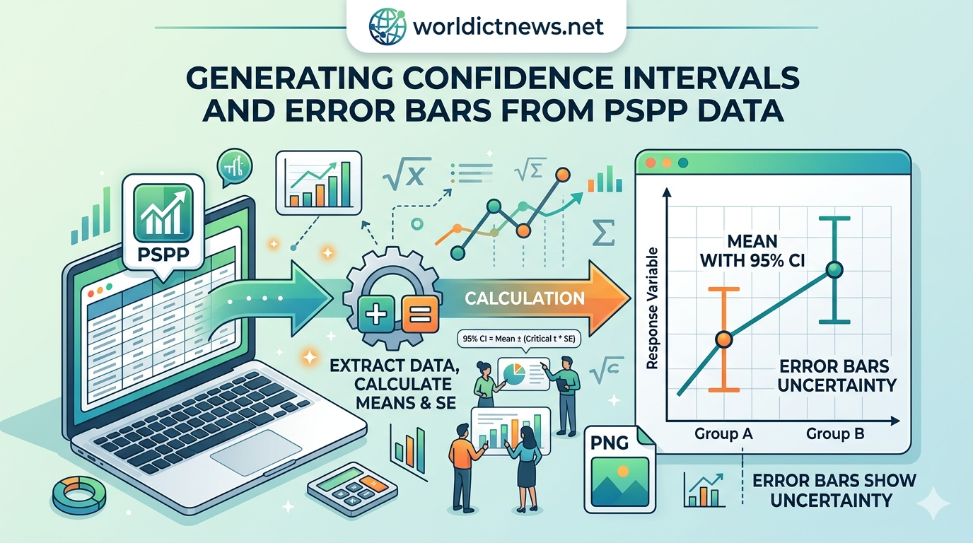
Table A: Descriptive Statistics Breakdown

This table outlines the essential parameters of the data distributions.

Financial Analysis:

• Large-Cap Equities generated the highest performance profile (\(\bar{X}_1 = 13.4\%\)).

• Corporate Bonds exhibited the lowest average performance profile (\(\bar{X}_2 = 5.5\%\)).

• REITs landed precisely in the middle tier (\(\bar{X}_3 = 9.9\%\)).

• The Standard Deviation columns illustrate underlying asset risks: Equities displayed the highest absolute internal volatility (\(1.306\%\)), while Bonds maintained tight, predictable clustering (\(0.524\%\)).

Table B: Checking the Homoscedasticity Guardrail

Before trusting the main F-statistic, we must verify the Homogeneity of Variance assumption using Levene’s Statistic.

Test of Homogeneity of Variances
Returns Annualized Performance (%)
+-------------------+-----+-----+-------+

| Levene Statistic  | df1 | df2 | Sig.  |
+-------------------+-----+-----+-------+

|       1.378       |  2  | 12  | 0.289 |
+-------------------+-----+-----+-------+

Statistical Rule:

• The crucial metric to inspect here is Sig. (which represents the exact p-value of Levene's Test).

• If the Levene p-value is greater than \(0.05\), we fail to reject the null hypothesis of equal variances. This confirms that the internal variances are sufficiently uniform, giving us the green light to proceed with standard ANOVA.

• Our Result: The Sig. value is \(0.289\). Since \(0.289 > 0.05\), the homoscedasticity assumption safely holds. [1]

Table C: Evaluating the Main ANOVA Matrix

This is the core ledger containing our calculated sums of squares, degrees of freedom, mean squares, and the calculated F-statistic. [1]

                                  ANOVA
Returns Annualized Performance (%)
+----------------+----------------+----+-------------+--------+-------+

|                | Sum of Squares | df | Mean Square |   F    | Sig.  |
+----------------+----------------+----+-------------+--------+-------+

| Between Groups |    156.100     |  2 |   78.050    | 79.949 | 0.000 |
| Within Groups  |     11.715     | 12 |    0.976    |        |       |
| Total          |    167.815     | 14 |             |        |       |
+----------------+----------------+----+-------------+--------+-------+

Final Step-by-Step Mathematical Validation:

Let us check the software calculations using our financial equations:

1. Degrees of Freedom (\(df\)):

   • \(df_{\text{Between}} = k - 1 = 3 - 1 = \mathbf{2}\)

   • \(df_{\text{Within}} = N - k = 15 - 3 = \mathbf{12}\)

   • \(df_{\text{Total}} = N - 1 = 15 - 1 = \mathbf{14}\)

2. Mean Squares (\(MS\)):

   • \(\text{MSB} = \frac{\text{SSB}}{df_{\text{Between}}} = \frac{156.100}{2} = \mathbf{78.050}\)

   • \(\text{MSW} = \frac{\text{SSW}}{df_{\text{Within}}} = \frac{11.715}{12} = \mathbf{0.976}\) [1, 2]

3. The F-Ratio:

   • \(F = \frac{\text{MSB}}{\text{MSW}} = \frac{78.050}{0.976} = \mathbf{79.949}\) [1]

The Decision Rule:

Look directly at the Sig. column (p-value) of the ANOVA output block. [1]

• If \(\text{Sig.} \le 0.05\), we reject the Null Hypothesis (\(H_{0}\)) and conclude that asset class choice significantly impacts investment performance.

• Our Result: The Sig. output displays \(0.000\) (which mathematically reads as \(p < 0.001\)).

Because the p-value is well below our significance threshold (\(0.05\)), we reject the null hypothesis. The empirical data proves that the average annualized historical returns across Large-Cap Equities, Corporate Bonds, and REITs are not equal.

7. Deep-Dive Post-Hoc Analysis

While the primary ANOVA omnibus test tells us that at least one asset class performs differently, it does not specify which pairs are driving the difference. To pinpoint where the significant outperformance lies, we turn to the Tukey Honestly Significant Difference (HSD) table generated by PSPP. [1]

                        Multiple Comparisons
Dependent Variable: Annualized Performance Return (%)
Tukey HSD
+--------------------+--------------------+-----------------+------------+-------+

| (I) Asset Class    | (J) Asset Class    | Mean Difference | Std. Error | Sig.  |
|     Category       |     Category       |     (I-J)       |            |       |
+--------------------+--------------------+-----------------+------------+-------+

| Large-Cap Equities | Corporate Bonds    |      7.900*     |   0.625    | 0.000 |
|                    | REITs              |      3.500*     |   0.625    | 0.000 |
+--------------------+--------------------+-----------------+------------+-------+

| Corporate Bonds    | Large-Cap Equities |     -7.900*     |   0.625    | 0.000 |
|                    | REITs              |     -4.400*     |   0.625    | 0.000 |
+--------------------+--------------------+-----------------+------------+-------+

| REITs              | Large-Cap Equities |     -3.500*     |   0.625    | 0.000 |
|                    | Corporate Bonds    |      4.400*     |   0.625    | 0.000 |
+--------------------+--------------------+-----------------+------------+-------+
* The mean difference is significant at the 0.05 level.

Interpretation of Pairwise Comparisons:

1. Large-Cap Equities vs. Corporate Bonds: The mean difference is \(+7.9\%\). The p-value (Sig.) is \(0.000\). Large-Cap Equities significantly outperform Corporate Bonds.

2. Large-Cap Equities vs. REITs: The mean difference is \(+3.5\%\). The p-value is \(0.000\). Large-Cap Equities significantly outperform REITs.

3. REITs vs. Corporate Bonds: The mean difference is \(+4.4\%\). The p-value is \(0.000\). REITs significantly outperform Corporate Bonds. [1]

Strategic Investment Takeaway

Every single asset class pair shows statistically significant performance boundaries. For the institutional endowment, this means that shifting capital between these three buckets will result in fundamentally distinct portfolio performance, rather than variance that could be erased by everyday market fluctuations.

8. Summary Checklist for Portfolio Analysts

To reliably scale this workflow for other financial datasets, keep this actionable summary checklist on hand:

  ┌────────────────────────────────────────────────────────┐
  │              FINANCIAL ANOVA CHECKLIST                 │
  ├────────────────────────────────────────────────────────┤
  │  1. VERIFY DATA STRUCTURE                              │
  │     - Dependent variable is continuous (e.g. Return)   │
  │     - Factor variable has 3+ groups (e.g. Sectors)     │
  │                                                        │
  │  2. RUN EXPLORATORY DESCRIPTIVES                       │
  │     - Check for data anomalies or entry typos          │
  │                                                        │
  │  3. ASSESS LEVENE'S TEST OUTPUT                        │
  │     - Is Sig. > 0.05?                                  │
  │       - YES: Proceed to standard ANOVA                 │
  │       - NO: Stop; use Welch adjustment instead         │
  │                                                        │
  │  4. EVALUATE OMNIBUS F-TEST                            │
  │     - Is Sig. <= 0.05?                                 │
  │       - YES: Reject Null; proceed to Post-Hoc          │
  │       - NO: Accept Null; no significant differences    │
  │                                                        │
  │  5. EXECUTE TUKEY HSD PAIRWISE                         │
  │     - Map out specific outperforming pairs             │
  │     - Inform final asset allocation strategy           │
  └────────────────────────────────────────────────────────┘

By substituting your own internal operational figures—such as risk-adjusted metrics, Sharpe ratios, or valuation multiples—into this PSPP workflow, you can back up your investment committees' asset allocation choices with clean, unassailable statistical proof.

9. Conclusion

ANOVA provides financial analysts and investment professionals with a robust framework to test hypotheses across multiple categories without inflating statistical error rates. By leveraging open-source tools like PSPP, teams can seamlessly run these advanced diagnostic workflows—from checking homoscedasticity via Levene's test to identifying outperformance using Tukey's HSD—without the overhead of proprietary software. Ultimately, integrating rigorous statistical verification into your analytical workflow transforms raw financial data into defensible, high-conviction investment strategies