Lecture Notes: Regression Analysis with Python by T. C. Okenna

Lecture Notes: Regression Analysis with Python.

By T. C. Okenna

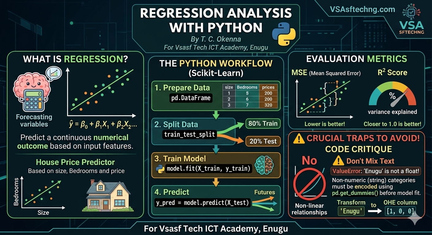
Regression Analysis is a fundamental statistical and machine learning technique used to model, investigate, and quantify the relationship between a dependent variable (target/outcome) and one or more independent variables (predictors/features).

📋 Lesson Overview

• Target Audience: Intermediate Python Learners & Aspiring Data Analysts

• Duration: 60 Minutes

• Prerequisites: Python fundamentals, core packages (Pandas, NumPy), and foundational algebra.

• Learning Objectives: By the end of this lesson, students will be able to:

  1. Differentiate between Simple and Multiple Linear Regression.

  2. Implement an end-to-end regression model pipeline using the Scikit-Learn Regression API.

  3. Interpret key parameters like coefficients, intercept, and evaluation metrics.

👩‍🏫 Lesson Structure

1. Introduction: The "Why" of Regression (10 Mins)

• The Real-World Analogy: Predicting your monthly electricity bill. The bill doesn't change randomly; it depends predictably on measurable factors like daily temperature, the square footage of your home, and the total runtime of your air conditioner.

• The Objective: We fit a line (or hyperplane) through data points so we can predict continuous numerical variables based on input inputs.

• The Mathematics:
  \(\^{y}=\beta {0}+\beta {1}X_{1}+\beta {2}X{2}+...+\beta {n}X{n}\)

  • \(\^{y}\): The predicted value (Dependent variable).

  • \(\beta _{0}\): The Intercept (Where the line crosses the y-axis when \(X=0\)).

  • \(\beta_1, \beta_2\): The Coefficients (The slope/weight showing how much \(y\) updates per unit change in \(X\)).

2. Core Concepts: Simple vs. Multiple Regression (10 Mins)

3. Step-by-Step Implementation with Python (25 Mins)

Here is a real-world coding solution predicting real estate prices based on spatial properties.

python

import numpy as np
import pandas as pd
from sklearn.model_selection import train_test_split
from sklearn.linear_model import LinearRegression
from sklearn.metrics import mean_squared_error, r2_score

# 1. Create a mock Real Estate dataset
data = {
    'Size_SqFt': [1500, 1800, 2400, 3000, 1200, 2100, 1600, 2800],
    'Bedrooms': [3, 3, 4, 4, 2, 3, 3, 4],
    'Price_USD': [250000, 290000, 380000, 470000, 190000, 330000, 265000, 430000]
}
df = pd.DataFrame(data)

# 2. Separate Features (X) and Target (y)
X = df[['Size_SqFt', 'Bedrooms']]
y = df['Price_USD']

# 3. Split dataset into Training (80%) and Testing (20%) sets
X_train, X_test, y_train, y_test =
train_test_split(X, y, test_size=0.2, random_state=42)

# 4. Instantiate and Train the Linear Regression Model
model = LinearRegression()
model.fit(X_train, y_train)

# 5. Generate Predictions using the test partition
y_pred = model.predict(X_test)

# 6. Extract Parameters
print(f"Intercept (Beta 0): {model.intercept_:.2f}")
print(f"Coefficients (Beta 1, Beta 2): {model.coef_}")

Use code with caution.

4. Evaluating Model Performance (10 Mins)

To measure how well our model fits the data, we use standard evaluation metrics:

• Mean Squared Error (MSE): Measures the average squared difference between actual values and predicted values. Lower is better.

• \(R^{2}\) Score (Coefficient of Determination): Represents the proportion of variance in the dependent variable that is predictable from the independent variables. Ranging from 0 to 1 (Higher is better, where 1.0 means a perfect fit).

python

# Continuing from the script above...
mse = mean_squared_error(y_test, y_pred)
r2 = r2_score(y_test, y_pred)

print(f"Mean Squared Error: {mse:.2f}")
print(f"R2 Score: {r2:.4f}")  # e.g., 0.9850 means 98.5% variance explained

Use code with caution.

5. ⚠️ Crucial Traps & Checklist (5 Mins)

When applying linear regression in production, look out for these pitfalls:

1. Non-Linear Relationships: Linear regression assumes a straight-line relationship. If your data bends dramatically, consider Polynomial features or alternate models.

2. Multicollinearity: If your independent variables (\(X_{1}\) and \(X_{2}\)) are highly correlated with each other (e.g., house size in square feet vs house size in square meters), it destabilizes coefficient tracking. Drop one of the redundant variables.

🎯 Diagnostic Challenge & Code Critique

Ask the Class: Look closely at this implementation fragment. What major data data structural mistake did the developer make before fitting the model?

python

import pandas as pd
from sklearn.linear_model import LinearRegression

# Loading regional sales logs
df = pd.DataFrame({
    'City': ['Enugu', 'Lagos', 'Abuja', 'Enugu'],
    'Marketing_Spend': [500, 1200, 900, 600],
    'Revenue': [4500, 11000, 8500, 5200]
})

X = df[['City', 'Marketing_Spend']]
y = df['Revenue']

model = LinearRegression()
model.fit(X, y) # 💥 CRASH!

Use code with caution.

Expected Solution Critique:

• The Error: This script throws a ValueError: could not convert string to float: 'Enugu'.

• The Reason: Linear regression is a purely mathematical optimization algorithm. It cannot handle raw string data like categorical city names directly.

• The Fix: Convert the string column into numerical vectors before fitting. Use data encoding techniques like One-Hot Encoding via pd.get_dummies(df, columns=['City']) to prepare it correctly.

For Vsasf Tech ICT Academy, Enugu