Machine Learning and Predictive Modeling Frameworks in Modern Data Science
Engines of Prediction: Machine Learning and Predictive Modeling Frameworks in Modern Data Science
At its core, data science transitions from an analytical discipline to an engineering powerhouse when it stops merely reporting the past and begins forecasting the future. Predictive modeling leverages structural patterns within historical data to build mathematical algorithms that can automatically classify categories or predict continuous trends. Rather than manually writing hardcoded business rules, engineers train machines to dynamically map complex features to real-world target variables.
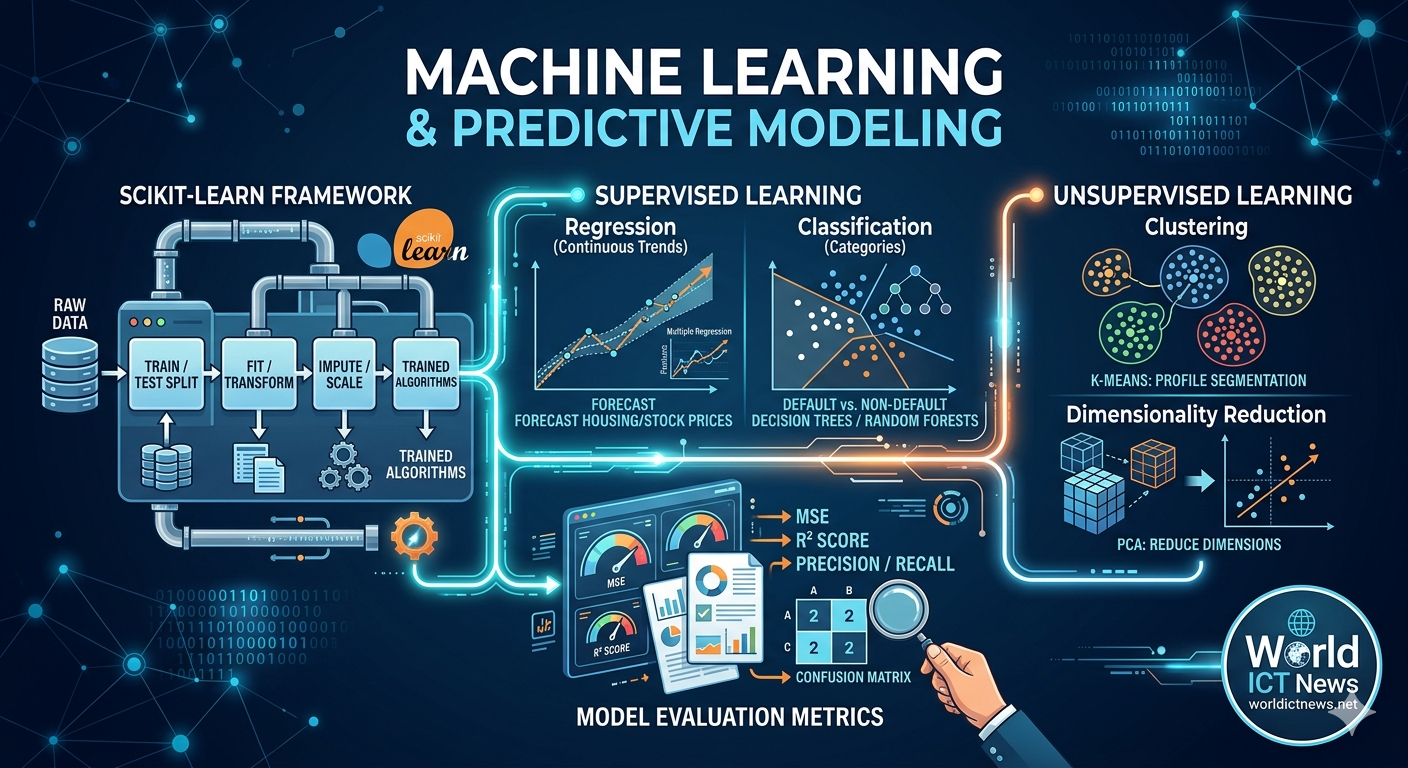
This comprehensive guide serves as an operational manual for constructing, executing, and evaluating modern machine learning pipelines. Using Scikit-Learn, the industry standard for production-grade modeling in Python, we will break down supervised regression and classification frameworks, map unsupervised clustering and dimensionality reduction paradigms, and establish the validation metrics required to keep production systems stable under changing market regimes.
1. The Scikit-Learn Framework: Building Robust, Production-Grade Data Pipelines
In production data science ecosystems, models fail not because of mathematical flaws, but due to architectural gaps. Issues like data leakage—where information from the future testing set accidentally bleeds into the training set—can invalidate an enterprise deployment. Scikit-Learn addresses this by providing a unified, object-oriented API built around three core design patterns:
Transformers: Objects that clean, scale, or modify data features (e.g.,
StandardScaler,OneHotEncoder). They implement a.fit()method to learn parameters from training data and a.transform()method to apply those changes.Estimators: The core machine learning models themselves (e.g.,
LinearRegression,RandomForestClassifier). They use.fit(X, y)to train on the data and find optimal internal parameters.Predictors: Trained estimators capable of generating inferences on unseen data through the
.predict(X)method.
The Anatomy of an End-to-End Pipeline
A production-grade machine learning lifecycle begins by isolating structural features from target vectors, followed immediately by a strict data split.
┌──────────────────────────────┐
│ Raw Dataset (X, y) │
└──────────────┬───────────────┘
│ (train_test_split)
┌──────────────┴──────────────┐
▼ ▼
[Training Set] [Testing Set]
(X_train, y_train) (X_test, y_test)
│ │
▼ │
Pipeline .fit() │
┌────────────────────────┐ │
│ 1. Impute Missing │ │
│ 2. Standard Scale │ │
│ 3. Train Model Weights │ │
└────────────────────────┘ │
│ ▼
└─────────────────────> Pipeline .predict()
│
▼
[Evaluation Metrics]
python
import numpy as np
import pandas as pd
from sklearn.model_selection import train_test_split
from sklearn.preprocessing import StandardScaler
from sklearn.impute import SimpleImputer
from sklearn.pipeline import Pipeline
from sklearn.compose import ColumnTransformer
# Create simulated enterprise operations data
np.random.seed(42)
n_records = 1000
data = {
'Operational_Age': np.random.randint(1, 15, n_records),
'Throughput_Rate': np.random.uniform(100.0, 500.0, n_records),
'Error_Count': np.random.poisson(lam=2, size=n_records),
'System_Failure': np.random.choice([0, 1], size=n_records, p=[0.85, 0.15])
}
df = pd.DataFrame(data)
# Introduce a few artificial missing values to simulate real-world data issues
df.iloc[np.random.choice(n_records, 20), 1] = np.nan
# Isolate features (X) from the target classification vector (y)
X = df.drop(columns=['System_Failure'])
y = df['System_Failure']
# Apply train_test_split immediately to prevent data leakage
X_train, X_test, y_train, y_test = train_test_split(X, y, test_size=0.2, random_state=42, stratify=y)
# Construct a preprocessing pipeline for continuous numeric features
numeric_features = ['Operational_Age', 'Throughput_Rate', 'Error_Count']
numeric_transformer = Pipeline(steps=[
('imputer', SimpleImputer(strategy='median')), # Replace missing NaNs safely
('scaler', StandardScaler()) # Scale features to zero mean and unit variance
])
# Combine transformers into a comprehensive column preprocessor
preprocessor = ColumnTransformer(
transformers=[('num', numeric_transformer, numeric_features)]
)
print(f"Training Features Shape: {X_train.shape}")
print(f"Testing Target Baseline Distribution:\n{y_test.value_counts(normalize=True)}")
Use code with caution.
2. Supervised Learning (Regression): Forecasting Continuous Metrics
Supervised learning applies when your target variable is fully labeled. When that target variable is a continuous quantitative value (such as a stock price, real estate valuation, or corporate revenue forecast), the problem is classified as a Regression task.
    [Simple Linear Regression]              [Multiple Linear Regression]
             Target (y)                              Target (y)
                ▲                                       ▲
                │      /                                │      /  /
                │    /                                  │    /  /
                │  /                                    │  /  /
                └──────────────►                        └──────────────►
                   Feature (X1)                            Features (X1, X2, X3)
             Single Predictor Variable               Multiple Predictor Features
Linear Regression
Linear regression models the relationship between a single predictor variable (X) and a continuous dependent variable (y) by fitting a linear equation to observed data. The equation is represented as:
\(y=\beta {0}+\beta {1}X+\epsilon \)
Where β₀ is the intercept, β₁ is the slope coefficient, and ε represents the residual error.
Multiple Linear Regression
In complex datasets, a target variable is rarely driven by a single feature. Multiple Linear Regression expands this formulation to include n distinct predictive dimensions:
\(y=\beta {0}+\beta {1}X_{1}+\beta {2}X{2}+\dots +\beta {n}X{n}+\epsilon \)
The algorithm uses Ordinary Least Squares (OLS) to minimize the sum of squared differences between actual data points and the predicted plane of best fit.
Data Science Context:
Regression models form the backbone of automated valuation platforms, asset depreciation tracking systems, and long-term demand planning modules.
python
from sklearn.linear_model import LinearRegression
from sklearn.metrics import mean_squared_error, r2_score
# Simulate real estate asset valuation parameters
np.random.seed(42)
square_footage = np.random.uniform(1200, 4500, 500)
num_bedrooms = np.random.randint(2, 6, 500)
distance_to_core_km = np.random.uniform(2, 35, 500)
# Generate a continuous target variable (Asset Price in USD) with random noise
asset_price_usd = (square_footage * 175) + (num_bedrooms * 25000) - (distance_to_core_km * 3200) + np.random.normal(0, 15000, 500)
df_housing = pd.DataFrame({
'Sq_Footage': square_footage,
'Bedrooms': num_bedrooms,
'Distance_Km': distance_to_core_km,
'Price_USD': asset_price_usd
})
# Separate into features and target matrix
X_reg = df_housing.drop(columns=['Price_USD'])
y_reg = df_housing['Price_USD']
X_train_r, X_test_r, y_train_r, y_test_r = train_test_split(X_reg, y_reg, test_size=0.2, random_state=42)
# Build a multiple linear regression workflow pipeline
reg_pipeline = Pipeline(steps=[
('scaler', StandardScaler()),
('regressor', LinearRegression())
])
# Train the OLS model weights
reg_pipeline.fit(X_train_r, y_train_r)
# Generate predictions on unseen data
y_pred_r = reg_pipeline.predict(X_test_r)
# Extract learned slope coefficients
coefficients = reg_pipeline.named_steps['regressor'].coef_
print("--- Supervised Multiple Regression Results ---")
for feat, coef in zip(X_reg.columns, coefficients):
print(f"Feature: {feat:<12} | Learned Weight Coefficient: {coef:>10.2f}")
Use code with caution.
3. Supervised Learning (Classification): Predicting Distinct Categorical Targets
When the target variable is categorical rather than continuous, the task shifts to Classification. The objective here is to assign observations to distinct, mutually exclusive buckets (e.g., flagging whether a loan application is a "default" vs. "non-default").
1. Logistic Regression
Despite its name, Logistic Regression is used for classification, not regression. Instead of drawing a straight line through points, it fits an S-shaped Sigmoid function that maps any continuous value to a probability between 0 and 1:
\(P(y=1|X)=\sigma (Z)=\frac{1}{1+e^{-Z}}\)
Where \(Z = \beta_0 + \beta_1 X_1 + \dots + \beta_n X_n\). If the probability passes a chosen threshold (usually 0.50), the system assigns the item to the positive class.
2. Decision Trees
Decision Trees segment data by sequentially splitting features based on criteria like Gini Impurity or Information Gain. The algorithm creates an intuitive tree structure of recursive conditional statements (e.g., “If Credit Score > 700 and Debt-to-Income Ratio < 0.35, then Approve”). While highly interpretable, individual decision trees are prone to overfitting—learning training noise so perfectly that they fail to generalize to new data.
3. Random Forests
To address the overfitting limitations of a single decision tree, Random Forests use an ensemble method called Bootstrap Aggregating (Bagging). The algorithm trains hundreds of independent decision trees in parallel, with each tree built on a random subset of the training data and features. The final classification is determined by a majority vote across all the individual trees. This ensemble approach cancels out individual errors, making Random Forests highly resilient models.
python
from sklearn.linear_model import LogisticRegression
from sklearn.tree import DecisionTreeClassifier
from sklearn.ensemble import RandomForestClassifier
# Construct a dictionary containing diverse classification architectures
classification_models = {
'Logistic_Regression': LogisticRegression(random_state=42),
'Decision_Tree': DecisionTreeClassifier(max_depth=5, random_state=42),
'Random_Forest': RandomForestClassifier(n_estimators=100, max_depth=8, random_state=42)
}
print("--- Initializing Classification Models Pipeline ---")
for model_name, model_obj in classification_models.items():
# Build a combined pipeline for each model using the preprocessor defined in Section 1
clf_pipeline = Pipeline(steps=[
('preprocessor', preprocessor),
('classifier', model_obj)
])
# Train the respective classifier
clf_pipeline.fit(X_train, y_train)
print(f"Successfully trained: {model_name}")
Use code with caution.
4. Unsupervised Learning: Clustering Unlabeled Patterns
In many real-world scenarios, datasets do not come with pre-labeled target variables. Unsupervised Learning algorithms analyze unlabelled data matrices to uncover hidden structures, group similar observations, or simplify complex features without human intervention.
       [ K-Means Clustering ]                [ Principal Component Analysis ]
               ▲                                            ▲
               │  ●   ●                                     │     ☼   ☼
               │    ○   ○                                   │   ☼  \ ☼
               │  ◌   ◌                                     │ ☼     \  ☼
               └──────────────►                             └──────────────►
         Groups data profiles into                    Projects high-dimensional space
         K distinct distance clusters                 onto principal orthogonal vectors
K-Means Clustering
K-Means groups data into K distinct clusters based on feature similarity. The algorithm operates through an iterative process:
It randomly places K centroids throughout the feature space.
It assigns each data point to its closest centroid using Euclidean distance.
It updates the centroid positions by calculating the mean coordinates of all assigned points.
It repeats this process until the centroids stabilize.
Principal Component Analysis (PCA)
High-dimensional datasets can overwhelm algorithms and obscure patterns—a challenge often referred to as the curse of dimensionality. PCA is a dimensionality reduction technique that transforms a large set of correlated variables into a smaller set of uncorrelated variables called Principal Components. It achieves this by projecting the data onto new orthogonal axes that capture the maximum possible variance, allowing you to compress features while retaining most of the underlying information.
python
from sklearn.cluster import KMeans
from sklearn.decomposition import PCA
# Generate unlabelled operational profiles for clustering evaluation
np.random.seed(42)
customer_spend = np.random.normal(200, 50, 300)
visit_frequency = np.random.normal(12, 4, 300)
support_tickets = np.random.normal(2, 1, 300)
X_unsupervised = pd.DataFrame({
'Spend': customer_spend,
'Frequency': visit_frequency,
'Tickets': support_tickets
})
# Standardize features before applying distance-based metrics
scaler = StandardScaler()
X_scaled = scaler.fit_transform(X_unsupervised)
# 1. Apply K-Means Clustering to segment customers into 3 behavioral profiles
kmeans = KMeans(n_clusters=3, random_state=42, n_init='auto')
X_unsupervised['Cluster_ID'] = kmeans.fit_predict(X_scaled)
# 2. Apply PCA to project 3-dimensional data down into a 2-dimensional plane
pca = PCA(n_components=2)
X_pca = pca.fit_transform(X_scaled)
print("--- Unsupervised Learning Output Profiles ---")
print(f"Total Explained Variance Ratio across top 2 PCA Components: {np.sum(pca.explained_variance_ratio_):.4f}")
print(X_unsupervised.groupby('Cluster_ID').mean())
Use code with caution.
5. Model Evaluation Metrics: Quantifying Performance Accuracy
A model is only as reliable as its validation framework. Evaluating performance requires selecting appropriate metrics that align with your specific business goals, rather than relying blindly on basic accuracy score readouts.
Regression Metrics
Mean Squared Error (MSE): Calculates the average of the squared differences between actual and predicted values. By squaring the errors, it heavily penalizes large outliers.
R-Squared (R²): Measures the proportion of variance in the dependent variable that can be explained by the independent features. An R² score of 1.0 indicates a perfect fit.
Classification Metrics
Confusion Matrix: A tabular layout that breaks down predictions into four cross-classified quadrants: True Positives (TP), False Positives (FP), True Negatives (TN), and False Negatives (FN).
Precision: Measures out of all positive predictions, how many were actually positive. It is the core metric to track when the cost of a false positive is exceptionally high (e.g., falsely accusing a legitimate transaction of fraud).
\(\text{Precision}=\frac{\text{TP}}{\text{TP}+\text{FP}}\)
Recall (Sensitivity): Measures out of all actual positive cases, how many the model successfully captured. This is the critical metric when false negatives carry severe consequences (e.g., failing to diagnose an illness or missing a critical system failure).
\(\text{Recall}=\frac{\text{TP}}{\text{TP}+\text{FN}}\)
python
from sklearn.metrics import classification_report, confusion_matrix
# Build, train, and validate a production-ready Random Forest Pipeline
prod_pipeline = Pipeline(steps=[
('preprocessor', preprocessor),
('rf_classifier', RandomForestClassifier(n_estimators=100, random_state=42))
])
prod_pipeline.fit(X_train, y_train)
y_pred = prod_pipeline.predict(X_test)
# Compute performance diagnostics
matrix_output = confusion_matrix(y_test, y_pred)
report_output = classification_report(y_test, y_pred, target_names=['Normal', 'Failure'])
print("--- Production Model Evaluation Diagnostic Metrics ---")
print("Confusion Matrix Layout Matrix:")
print(matrix_output)
print("\nComprehensive Classification Validation Ledger:")
print(report_output)
Use code with caution.
6. End-to-End Operational Validation Checklist
To consistently scale machine learning architectures across disparate business environments, use this engineering checklist:
Operational Phase | Critical Validation Questions | Scikit-Learn Module Component | Common Warning Flags |
|---|---|---|---|
Pipeline Splits | Is your testing data securely isolated from training data before preprocessing? |
| Unusually high performance metrics |
Feature Scaling | Have feature scales been normalized so distance calculations remain balanced? |
| K-Means models tracking a single feature |
Imputation Safety | Are missing values handled safely using localized training parameters? |
| Data leakage across validation bounds |
Supervised Choice | Are continuous metrics routed to regression models and categories to classifiers? |
| Classification metrics on floats |
Metric Alignment | Does your evaluation strategy prioritize Precision or Recall based on business risk? |
| Maximizing accuracy while ignoring high false negatives |
7. Conclusion
Building a successful machine learning pipeline requires balancing theoretical statistical principles with clean, repeatable software architecture. Scikit-Learn simplifies this process by allowing engineers to bundle missing data handling, feature scaling, and predictive modeling into a single, cohesive workflow object.
Whether you are building multiple regression models to project financial assets, deploying random forest ensembles to catch system anomalies, or using PCA to compress complex datasets, success ultimately hinges on rigorous validation. Clear metrics—such as precision, recall, and explained variance—transform abstract algorithms into reliable data assets for the modern enterprise.
Did you find this ICT insight helpful?