The Latest in

Master Chi-Square Calculations in PSPP: A Step-by-Step Guide with Practical Examples. In statistical analysis, understanding relationships between categorical variables is a fundamental requirement across disciplines—ranging from public health and marketing research to social sciences and quality control. While commercial software packages like IBM SPSS are widely used for this purpose, their steep licensing costs often present a barrier to students, independent researchers, and non-profit organizations.Fortunately, PSPP offers a powerful, completely free, and open-source alternative. Designed as a drop-in replacement for SPSS, PSPP replicates its user interface, command syntax, and data handling logic.This comprehensive guide will walk you through the theory and practical execution of Chi-Square (\(\chi ^{2}\)) tests using PSPP. We will explore both the Goodness-of-Fit Test and the Test of Independence using clear, step-by-step examples.1. Understanding the Core Concepts of Chi-Square TestsBefore opening PSPP, it is critical to understand what a Chi-Square test does and when it should be applied. Chi-Square tests are non-parametric statistics, meaning they do not assume your data follows a normal distribution curve. Instead, they operate purely on frequencies (counts) within nominal or ordinal categorical data.There are two primary flavors of the Chi-Square test, each answering a distinct research question:A. The Chi-Square Goodness-of-Fit TestThis test evaluates a single categorical variable. It determines whether the observed distribution of data points across various categories matches an expected distribution (such as an equal split or a distribution derived from historical census data).Research Question Example: Does a retail store attract an equal number of customers on every day of the week?B. The Chi-Square Test of Independence (Crosstabulation)This test evaluates two categorical variables simultaneously. It determines whether there is a statistically significant association between them, essentially checking if the distribution of one variable depends on the categories of the second variable.Research Question Example: Is there a relationship between a person’s employment status (Employed vs. Unemployed) and their preferred mode of public transit (Bus, Train, or Taxi)?Crucial Assumptions for All Chi-Square TestsTo ensure your PSPP output is valid, your dataset must meet these core assumptions:Categorical Data: Variables must be nominal (e.g., gender, region) or ordinal (e.g., satisfaction level: low, medium, high).Independence of Observations: Each subject or data point must occupy exactly one cell. You cannot have the same person counted multiple times across different categories.Adequate Sample Size: A classic rule of thumb is that the expected frequency in any given cell should be 5 or greater for at least 80% of the cells. If your expected counts are too low, the test loses statistical power and accuracy.2. Preparing and Structuring Data in PSPPTo follow along with our upcoming examples, you must understand how data can be entered into PSPP. PSPP allows for two distinct entry formats: Raw Individual Data and Weighted Aggregated Data.Approach A: Entering Raw Individual DataIn this format, each row in your PSPP Data View represents a single, unique participant or observation. If you surveyed 150 people, your spreadsheet will have exactly 150 rows.Example Columns: Participant_ID, Gender, Job_Satisfaction.Approach B: Entering Weighted Aggregated Data (Time-Saver)If you already possess a summarized tally table (e.g., from a report), you do not need to manually type 150 rows. Instead, you create a summary grid with a dedicated Weight Variable.Example Columns: Gender, Job_Satisfaction, and Count.How to Activate Weighting in PSPP:If using Approach B, you must explicitly tell PSPP to treat your count column as a multiplier.Navigate to the top menu and select Data \(\rightarrow \) Weight Cases...In the dialog box that appears, select the radio button for Weight cases by.Move your summary frequency variable (e.g., Count) into the Frequency Variable slot.Click OK. A small indicator reading "Weight On" will appear in the bottom-right status bar of your PSPP window.3. Example 1: Chi-Square Goodness-of-Fit TestScenarioA university student council claims that student enrollment across four major academic tracks—Science, Arts, Business, and Engineering—is perfectly balanced, with an equal 25% distribution in each stream. A researcher collects a random sample of 200 students to test this hypothesis.Hypothesis FormulationNull Hypothesis (\(H_{0}\)): Student enrollment is uniformly distributed across all four academic tracks (Observed Frequencies = Expected Frequencies).Alternative Hypothesis (\(H_{1}\)): Student enrollment is not uniformly distributed across the tracks; a preference pattern exists.Step-by-Step Execution in PSPPStep 1: Variable and Data EntryOpen PSPP and switch to the Variable View tab at the bottom left. Define your variable:Name: TrackType: NumericLabel: Academic TrackValue Labels: Click the cell to define your categories:1 = Science2 = Arts3 = Business4 = EngineeringSwitch to the Data View tab. We will use the weighted frequency method for swift input. Create a second variable named Frequency, turn on Weight Cases, and enter the following counts:Science (1): 65 studentsArts (2): 35 studentsBusiness (3): 40 studentsEngineering (4): 60 students[Data View Layout]Track | Frequency---------------------1.00 | 65.002.00 | 35.003.00 | 40.004.00 | 60.00Step 2: Running the AnalysisGo to the top navigation bar and select: Analyze \(\rightarrow \) Non-Parametric Tests \(\rightarrow \) Chi-Square...A dialog box will open. Select your variable Academic Track [Track] from the left panel and click the arrow button to move it into the Test Variable List.Under the Expected Values section, leave the default option selected: All categories equal (since our null hypothesis tests an equal 25% split).Click OK.+-------+| Chi-Square Test |+--------+| Test Variable List: Expected Values: || +-------+ (x) All categories equal|| | [Track] | ( ) Values: [ ] || +-------+ |+----------+Interpreting the Output WindowPSPP will launch its Output Viewer window containing two primary tables:Table 1: FrequenciesThis table displays your category names alongside three crucial metrics: Observed N (your actual data: 65, 35, 40, 60), Expected N (calculated by dividing the total sample of 200 by 4 categories, yielding 50 per cell), and the Residual (Observed minus Expected).Table 2: Test StatisticsThis contains the mathematical conclusion of your test:Chi-Square Value: \(\chi^2 = 14.00\)Degrees of Freedom (df): Calculated as \(k - 1\) (where \(k\) is the number of categories). \(4 - 1 = 3\).Asymp. Sig. (p-value): This is the most critical number for decision-making. Let us assume it reads 0.003.+-----------------------------------+| Test Statistics |+-----------------------------------+| Chi-Square | 14.000 || df | 3 || Asymp. Sig. | 0.003 |+-----------------------------------+Statistical ConclusionBecause our asymptotic significance value (\(p = 0.003\)) is substantially lower than our standard alpha threshold of \(0.05\), we reject the null hypothesis (\(H_{0}\)).Reporting the result: "A Chi-Square Goodness-of-Fit test indicated that student enrollment was not equally distributed across academic tracks, \(\chi^2(3) = 14.00, p < 0.01\)." The data shows that Science and Engineering tracks have higher enrollment numbers than expected, while Arts and Business lag behind.4. Example 2: Chi-Square Test of Independence (Two Variables)ScenarioA public health organization wants to know whether there is an association between an individual's Physical Activity Level (Sedentary vs. Active) and their self-reported Sleep Quality (Poor, Average, Good). They survey a sample of 300 adults.Hypothesis FormulationNull Hypothesis (\(H_{0}\)): Physical activity level and sleep quality are independent of one another (no relationship exists).Alternative Hypothesis (\(H_{1}\)): Physical activity level and sleep quality are dependent/associated with one another.Step-by-Step Execution in PSPPStep 1: Define VariablesOpen a new dataset tab in PSPP and navigate to Variable View. Configure three distinct variables:Name: ActivityLabel: Physical Activity LevelValue Labels: 1 = Sedentary, 2 = ActiveName: SleepLabel: Sleep QualityValue Labels: 1 = Poor, 2 = Average, 3 = GoodName: CountLabel: Number of Respondents (Remember to apply Data \(\rightarrow \) Weight Cases using this variable!)Step 2: Populate the Data MatrixSwitch over to Data View. Because we have 2 activity levels multiplied by 3 sleep tiers, we must enter all 6 unique combinations along with their aggregated counts:Activity | Sleep | Count------------------------------1 (Seden) | 1 (Poor) | 55.001 (Seden) | 2 (Aver) | 60.001 (Seden) | 3 (Good) | 35.002 (Active) | 1 (Poor) | 25.002 (Active) | 2 (Aver) | 65.002 (Active) | 3 (Good) | 60.00Step 3: Executing the Crosstabs ProcedureNavigate to the top menu option: Analyze \(\rightarrow \) Descriptive Statistics \(\rightarrow \) Crosstabs...A configuration panel will populate.Select Physical Activity Level [Activity] from your variable repository and transfer it to the Row(s) box using the corresponding arrow button.Select Sleep Quality [Sleep] and transfer it into the Column(s) box.Click the Statistics... button located at the bottom of the dialog window. Check the box labeled Chi-square, then click Continue.(Optional but highly recommended) Click the Cells... button. Under Counts, make sure Observed and Expected are both selected. This step helps you easily verify the "minimum cell count of 5" assumption. Click Continue.Click OK to process.+-------+| Crosstabs |+------+| Variables: Row(s): || +-----+ +------+ || | | --> | [Activity] | || +-----+ +----+ || Column(s): || +-----+ || | [Sleep] | || +-----+ || [Statistics...] (Chi-Square checked) |+--------+Interpreting the Output WindowYour PSPP Output Viewer will generate three core panels:1. Case Processing SummaryThis simple tracking card displays the sample breakdown. It confirms that 100% of your 300 targeted analytical cases were safely captured without encountering missing cell exclusions.2. Activity * Sleep CrosstabulationBecause we enabled Expected Counts, each intersection square will contain two data values:Observed Count: The real-world data points we manually entered.Expected Count: What the software calculates assuming no relationship exists between exercise and sleep. For instance, notice that for the Sedentary \(\times \) Poor Sleep intersection, the observed count (55) is noticeably higher than the mathematically expected baseline pattern (40.0).3. Chi-Square Tests TableLook closely at the row header designated as Pearson Chi-Square:+-------+| Chi-Square Tests |+--------+| | Value | df | Asymp. Sig. (2- || | | | sided) |+----+---+---+----+| Pearson Chi-Square | 17.216 | 2 | 0.000 || N of Valid Cases | 300 | | |+--------+Value: The calculated test statistic (\(\chi^2 = 17.216\)).df (Degrees of Freedom): Calculated using the formula \((R - 1) \times (C - 1)\), where \(R\) equals rows and \(C\) equals columns. For our layout: \((2 - 1) \times (3 - 1) = 1 \times 2 = 2\).Asymp. Sig. (2-sided): The calculated probability value (\(p = 0.000\)). Note that in statistical output, 0.000 does not mean zero probability; it means the p-value is extremely small (\(p < 0.001\)).Statistical ConclusionBecause our calculated asymptotic significance value (\(p < 0.001\)) falls comfortably below the critical \(0.05\) threshold, we reject the null hypothesis (\(H_{0}\)).Reporting the result: "A Pearson Chi-Square Test of Independence demonstrated a statistically significant association between an individual's physical activity level and their reported sleep quality, \(\chi^2(2) = 17.22, p < 0.001\)."By cross-referencing our observed versus expected cell counts, we can infer that sedentary individuals experience a disproportionately higher rate of poor sleep quality, whereas active individuals achieve average or good sleep marks at rates higher than expected.5. Troubleshooting Common Errors in PSPPWhen conducting Chi-Square procedures inside PSPP, you may occasionally encounter error notifications or confusing outputs. Use this quick reference guide to resolve common issues:Issue A: The output table displays fractional frequencies (e.g., 23.40 rows)The Cause: You forgot to turn off the Weight Cases tool from a previous analytical run, or you selected an incorrect weighting variable column.The Fix: Go to Data \(\rightarrow \) Weight Cases, choose the radio button for Do not weight cases, and click OK to reset your configuration baseline.Issue B: The Asymptotic Significance value reads completely blank or returns .The Cause: This occurs if your dataset lacks data variation, such as entering data where all respondents select a single option. This results in a matrix with 0 degrees of freedom, making division operations mathematically impossible.The Fix: Double-check your data layout in Data View. Ensure you have entered your value categories and counts correctly across distinct categorical rows.Issue C: A warning note states "Expected values are less than 5"The Cause: Your overall sample size is too small, or your data points are distributed across too many complex categorical choices. This directly violates our minimum cell size assumption.The Fix: You must collect a larger data sample, or combine related low-frequency categories to simplify your matrix. For example, you could merge an "Extremely Dissatisfied" choice category into a broader "Dissatisfied" group using the Transform \(\rightarrow \) Recode into Different Variables utility.

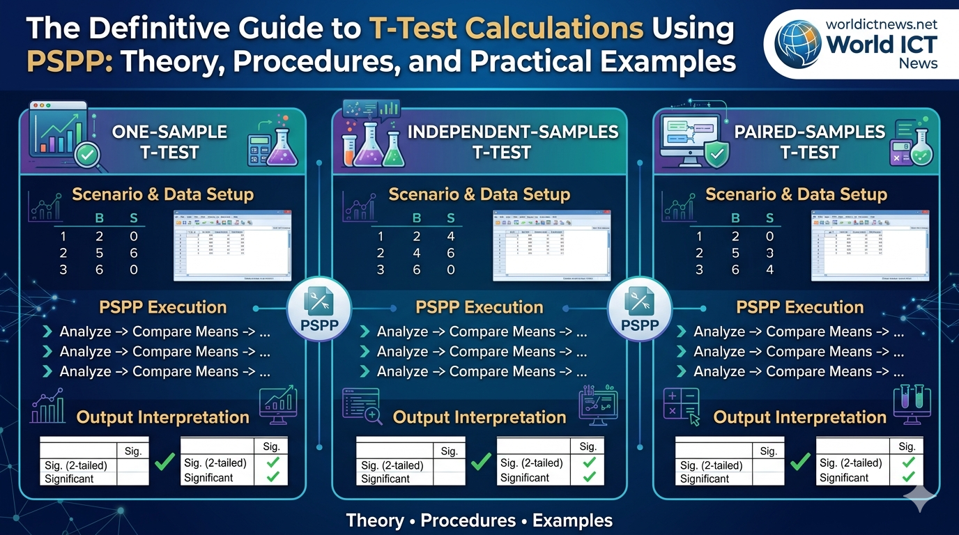
The Definitive Guide to T-Test Calculations Using PSPP: Theory, Procedures, and Practical Examples. IntroductionIn quantitative research, comparing the mean scores of different groups or conditions is a fundamental task. Researchers often need to determine if an observed difference between two averages is statistically meaningful or simply a result of random sampling variation. To answer this question, analysts rely on the T-Test, a family of parametric statistical tests developed by William Sealy Gosset under the pseudonym "Student."While commercial statistical software suites like IBM SPSS are widely used for these calculations, their prohibitive licensing costs present significant barriers for independent researchers, students, and institutions in developing regions. PSPP serves as a powerful, free, open-source alternative. It mirrors the user interface, functionalities, and syntax language of SPSS, allowing users to execute complex statistical analyses seamlessly.This comprehensive guide provides step-by-step procedures for calculating the three primary types of T-Tests using PSPP: One-Sample T-Tests, Independent-Samples T-Tests, and Paired-Samples (Dependent) T-Tests. Each procedure is accompanied by a practical research scenario, a concrete example dataset, step-by-step data configuration instructions, and a framework for output interpretation.1. Fundamentals of the T-Test FamilyBefore executing commands in PSPP, it is vital to understand which T-Test fits your research design. All T-Tests compare means, but they differ based on where the data originates.The Three Varieties of T-TestsOne-Sample T-Test: Compares the mean of a single sample against a known or predetermined population mean or hypothetical test value.Independent-Samples T-Test: Compares the means of two distinct, unrelated groups (e.g., males vs. females, treatment group vs. control group) on the same continuous variable.Paired-Samples T-Test (Dependent T-Test): Compares the means of the same group of subjects at two different points in time or under two different conditions (e.g., pre-test vs. post-test scores).Core Statistical AssumptionsTo ensure the mathematical validity of your T-Test results in PSPP, your dataset should satisfy the following parameters:Continuous Scale: The dependent variable must be measured at the interval or ratio level.Independence of Observations: There must be no relationship between the observations within each group (crucial for Independent T-Tests).Normal Distribution: The dependent variable should be approximately normally distributed within each group.Homogeneity of Variance: For independent designs, the variances of the two groups should be roughly equal (tested via Levene's Test in PSPP).2. Procedure 1: One-Sample T-TestScenario & Example DatasetA university claims that its graduating seniors spend an average of 15 hours per week studying outside of class. A student researcher suspects the actual study time is different. They collect data from 8 randomly selected seniors.Hypothetical Population Mean (Test Value): 15Sample Data (Hours per week): 12, 14, 18, 11, 13, 16, 12, 10Data Entry in PSPPLaunch PSPP and select the Variable View tab at the bottom left.In row 1, type Study_Hours under the Name column. Set Decimals to 0 and type Weekly Study Hours under Label.Switch to the Data View tab.In the Study_Hours column, enter the 8 data points vertically into rows 1 through 8.Study_Hours ----------- 12 14 18 11 13 16 12 10 Execution StepsNavigate to the top menu bar and select Analyze \(\rightarrow \) Compare Means \(\rightarrow \) One Sample T Test...A dialog box will open. Select Weekly Study Hours [Study_Hours] from the left panel and click the arrow button (\(\rightarrow \)) to move it into the Test Variable(s) window.Locate the field labeled Test Value at the bottom of the box. Delete the default 0 and type 15.Click OK.Output InterpretationPSPP will display two tables in the Output Viewer: "One-Sample Statistics" and "One-Sample Test". One-Sample Statistics============Variable | N | Mean | Std. Deviation | SE. Mean----+-----+----+----+-----Weekly Study Hours | 8 | 13.25 | 2.60 | 0.92============= One-Sample Test==============Test Value = 15---------------- | | | | Mean | 95% Conf. Int.Variable | t | df | Sig. | Difference | Lower | Upper---+--+--+---+----+--+---Weekly Study Hours | -1.90| 7 | 0.100 | -1.75 | -3.92 | 0.42=============Mean: The sample mean is 13.25 hours, which is lower than the claimed 15 hours.t-value: The calculated test statistic is -1.90.df (Degrees of Freedom): Calculated as \(N - 1 = 7\).Sig. (2-tailed): This is your p-value, which is 0.100.Statistical Decision: Because the p-value (\(0.100\)) is greater than the standard significance threshold (\(\alpha = 0.05\)), you fail to reject the null hypothesis. The difference between the sample mean (13.25) and the claimed mean (15) is not statistically significant.3. Procedure 2: Independent-Samples T-TestScenario & Example DatasetAn instructional designer wants to evaluate if a new interactive e-learning platform results in higher exam scores compared to traditional textbook learning. They test two independent groups of students.Group 1 (Textbook): 5 studentsGroup 2 (E-Learning): 5 studentsDependent Variable: Test Score (out of 100)Group 1 (Textbook) ScoreGroup 2 (E-Learning) Score75, 82, 78, 70, 8085, 89, 94, 80, 88Data Entry in PSPPUnlike spreadsheets where groups are placed side-by-side, statistical packages require a Grouping Variable (categorical code) and a Test Variable (continuous data).In Variable View, define two variables:Row 1: Name = Method, Type = Numeric, Decimals = 0, Label = Instructional Method.Row 2: Name = Score, Type = Numeric, Decimals = 0, Label = Exam Score.Click on the Value Labels cell for the Method variable. Define the groups:Value: 1 \(\rightarrow \) Label: Textbook \(\rightarrow \) Click Add.Value: 2 \(\rightarrow \) Label: E-Learning \(\rightarrow \) Click Add \(\rightarrow \) Click OK.Switch to Data View and arrange the 10 cases vertically:Method | Score -------+------- 1 | 75 1 | 82 1 | 78 1 | 70 1 | 80 2 | 85 2 | 89 2 | 94 2 | 80 2 | 88 Execution StepsSelect Analyze \(\rightarrow \) Compare Means \(\rightarrow \) Independent-Samples T Test...Move Exam Score [Score] into the Test Variable(s) window.Move Instructional Method [Method] into the Grouping Variable box.Notice that the Define Groups button becomes clickable. Click it.Type 1 into Group 1 and 2 into Group 2. Click Continue.Click OK.Output InterpretationThe Output Viewer yields a group breakdown and a comprehensive split test matrix. Group Statistics=========Method | N | Mean | Std. Deviation | SE. Mean--+-+--+--+-----Textbook | 5 | 77.00 | 4.64 | 2.07E-Learning | 5 | 87.20 | 5.12 | 2.29========== Independent Samples Test=========Levene's Test for Equality of Variances: F = 0.081 | Sig. = 0.784------------- | t | df | Sig.(2-tail) | Mean Difference--+--+--+-+---Equal var. assumed | -3.31 | 8 | 0.011 | -10.20Equal var. not assumed| -3.31 | 7.92 | 0.011 | -10.20==========Step 1: Check Levene's Test. Look at Sig. = 0.784. Because this value is much greater than \(0.05\), the variances are equal. We read the data from the row labeled Equal variances assumed.t-value and df: \(t = -3.31\) with \(8\) degrees of freedom.Sig. (2-tailed): The p-value is 0.011.Statistical Decision: Since \(0.011 < 0.05\), the result is statistically significant. The E-Learning group achieved a significantly higher mean test score (\(87.20\)) compared to the Textbook group (\(77.00\)).4. Procedure 3: Paired-Samples T-TestScenario & Example DatasetA medical clinic evaluates a new 4-week exercise regimen designed to reduce systolic blood pressure. The researcher records the blood pressure of 6 participants before starting the program and immediately after completion.ParticipantPre-Test Score (mmHg)Post-Test Score (mmHg)114513821381323150142416015151351366142139Data Entry in PSPPBecause the samples are paired (dependent), each row must represent an individual subject with both measurements placed side-by-side.In Variable View, define two variables:Row 1: Name = Pre_BP, Label = Systolic BP BeforeRow 2: Name = Post_BP, Label = Systolic BP AfterSwitch to Data View and enter the data across 6 rows:Pre_BP | Post_BP -------+-------- 145 | 138 138 | 132 150 | 142 160 | 151 135 | 136 142 | 139 Execution StepsNavigate to Analyze \(\rightarrow \) Compare Means \(\rightarrow \) Paired-Samples T Test...Click on Systolic BP Before [Pre_BP] and then click on Systolic BP After [Post_BP].Click the arrow button (\(\rightarrow \)) to move the selected combination into the Paired Variables window as a linked pair (Pre_BP - Post_BP).Click OK.Output Interpretation Paired Samples Statistics=========Variable | N | Mean | Std. Deviation | SE. Mean---+-+--+--+---Systolic BP Before | 6 | 145.33 | 8.78 | 3.58Systolic BP After | 6 | 139.67 | 6.47 | 2.64========== Paired Samples Test========= | | | | Mean | 95% Conf. Int.Pair 1 | t | df | Sig.2 | Diff. | Lower | Upper-+-+-+-+--+--+--Pre_BP - Post_BP | 4.11 | 5 | 0.009 | 5.67 | 2.12 | 9.21==========Means Comparison: The mean blood pressure dropped from 145.33 mmHg before the program to 139.67 mmHg after.Mean Difference: The average net reduction per person was 5.67 mmHg.t-value and df: \(t = 4.11\) with \(5\) degrees of freedom.Sig. (2-tailed): The p-value is 0.009.Statistical Decision: Since \(0.009 < 0.05\), the drop in blood pressure is statistically significant. The 4-week exercise program is an effective intervention for lowering systolic blood pressure.5. Alternative Execution: Using PSPP Syntax WorkspaceIf you want to bypass the graphical user interface or run your data analysis via scripting for reproducibility, you can use PSPP Syntax.Open a new window by choosing File \(\rightarrow \) New \(\rightarrow \) Syntax.Depending on your chosen analysis, paste one of the following code blocks:spss* --- COMMAND FOR ONE-SAMPLE T-TEST ---T-TEST /TESTVAL=15 /VARIABLES=Study_Hours.* --- COMMAND FOR INDEPENDENT-SAMPLE T-TEST ---T-TEST /GROUPS=Method(1, 2) /VARIABLES=Score.* --- COMMAND FOR PAIRED-SAMPLES T-TEST ---T-TEST /PAIRS=Pre_BP WITH Post_BP (PAIRED).Use code with caution.Highlight the desired block of text and select Run \(\rightarrow \) Selection from the top menu.6. Troubleshooting Common PSPP ErrorsMissing Variables in the Selection Panels: If your variable does not appear in the T-Test selection list, check its Type in Variable View. String (text) variables cannot be used in mathematical mean comparisons. Change the type to Numeric.Incorrect Levene's Row Choice: For the Independent T-Test, if Levene’s test value Sig. is less than 0.05, you must reject the assumption of variance equality. In that case, read the metrics from the bottom row, labeled Equal variances not assumed (Welch's T-test adjustment).Empty Output Matrix: Ensure your variables do not contain non-numeric characters or unmapped values. PSPP will drop incomplete data points listwise, resulting in empty values if your datasets are small.ConclusionMastering the execution of T-Tests within PSPP allows you to make data-driven comparisons without relying on expensive software. Whether checking a single group against a standard benchmark, evaluating two distinct educational methods, or observing variations over time, following these structured procedures ensures accurate results and clear reporting for your research project.

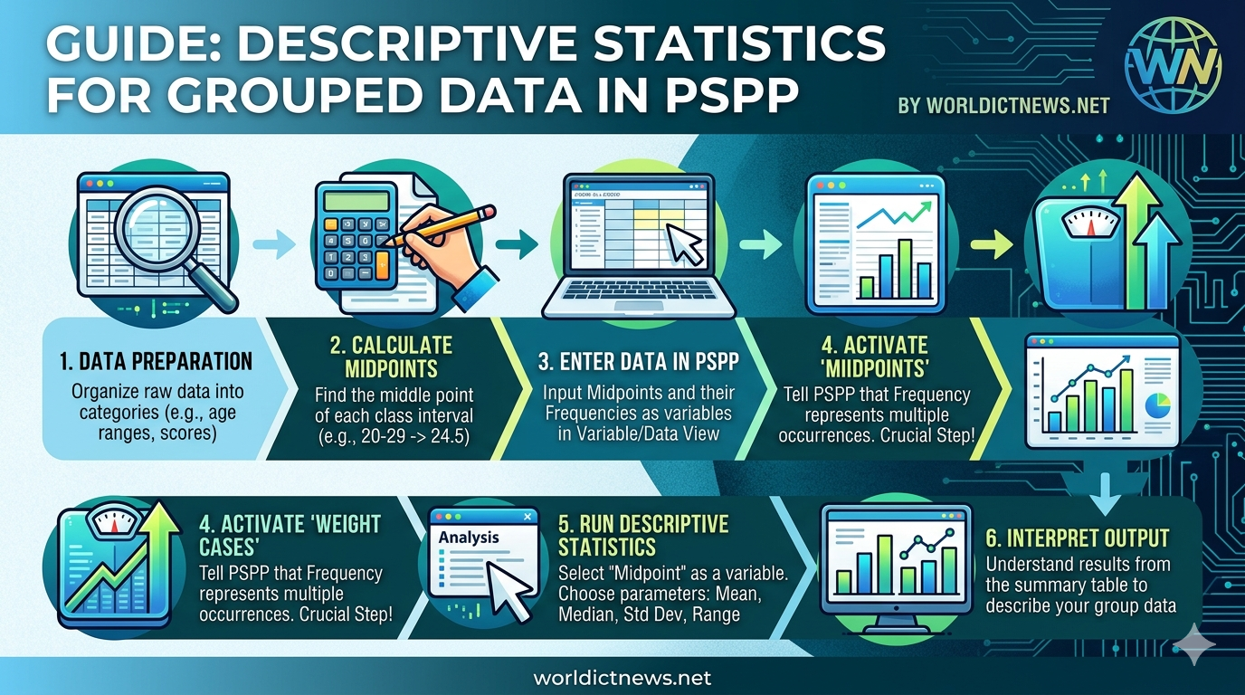
Master Guide: Calculating Descriptive Statistics for Grouped Data Using PSPP. IntroductionIn data analysis, we often encounter datasets where individual raw scores are unavailable. Instead, the data is pre-arranged into intervals, ranges, or categories. This format is known as grouped data. Grouped data is highly efficient for summarizing massive datasets, tracking frequency distributions, and understanding demographic spreads. However, analyzing grouped data requires a fundamentally different statistical approach than analyzing unorganized raw data.To analyze this data without expensive software licenses, researchers turn to PSPP. PSPP is a powerful, open-source alternative to IBM SPSS. It replicates the SPSS user interface and syntax, making high-level statistical analysis accessible to everyone.This comprehensive article provides a step-by-step procedure for calculating descriptive statistics for grouped data using PSPP. You will learn how to structure your dataset, apply essential statistical adjustments, and interpret your output data effectively.1. Understanding Descriptive Statistics for Grouped DataWhen dealing with ungrouped data, computing the mean, median, or standard deviation is straightforward. You simply add up the scores or look for the exact middle value. With grouped data, individual identities are lost inside class intervals (e.g., ages 20–29, 30–39).To calculate statistics for grouped data, we must work with two primary components:Class Midpoints (\(X_{m}\)): The exact middle value of a class interval. This serves as the proxy value for all individual scores contained within that group.Frequencies (\(f\)): The number of observations or participants falling inside that specific interval.Statistical Adjustments in PSPPSoftware packages like PSPP are naturally built to calculate descriptive statistics from individual case rows. If you enter grouped data into PSPP normally, the software will read your frequencies as single, independent data points rather than group multipliers. To fix this, we must use a critical feature called Weight Cases. This instructs PSPP to treat your frequency column as a scale multiplier, ensuring your mean, variance, and standard deviation calculations are mathematically accurate for the total population size (\(N = \sum f\)).2. Preparing and Formatting Grouped Data for PSPPBefore launching PSPP, you must structure your grouped data correctly. Let us look at a practical sample scenario: analyzing the monthly operational costs of 50 small tech startups.Class Interval (Cost in USD)Frequency (Number of Startups)$1,000 – $2,0008$2,001 – $3,00015$3,001 – $4,00018$4,001 – $5,0009Step 1: Calculate the Class Midpoints ManuallyStandard statistical software cannot natively process a text range (like "$1,000 – $2,000") as a mathematical value. You must calculate the midpoint for each interval before data entry.\(\text{Midpoint\ }(X_{m})=\frac{\text{Lower\ Limit}+\text{Upper\ Limit}}{2}\)For Interval 1: \((1000 + 2000) / 2 = \mathbf{1500}\)For Interval 2: \((2001 + 3000) / 2 = \mathbf{2500.5}\) (Rounded to 2501 for ease)For Interval 3: \((3001 + 4000) / 2 = \mathbf{3500.5}\) (Rounded to 3501)For Interval 4: \((4001 + 5000) / 2 = \mathbf{4501}\)Step 2: Set Up Your Cleaned Data TableYour adjusted table, ready for software input, will look like this:Midpoint (\(X_{m}\))Frequency (\(f\))15008250115350118450193. Step-by-Step Data Entry in PSPPWith your midpoints calculated, it is time to input this information into PSPP.Step 1: Define the VariablesLaunch PSPP.Look at the bottom-left corner of the interface and click on the Variable View tab.In the first row under the Name column, type Midpoint and press Enter.In the second row under the Name column, type Frequency and press Enter.Keep the Type set to Numeric for both variables.Set the Decimals column to 0 for clean numerical viewing.Under the Label column, provide descriptive definitions for clarity:For Midpoint, type: Estimated Class Midpoint (USD)For Frequency, type: Number of Startup ObservationsStep 2: Populate the DatasetSwitch to the Data View tab at the bottom-left corner of the screen.You will now see two columns labeled Midpoint and Frequency.Carefully type your calculated data matrix into the rows:Row 1: 1500 under Midpoint | 8 under FrequencyRow 2: 2501 under Midpoint | 15 under FrequencyRow 3: 3501 under Midpoint | 18 under FrequencyRow 4: 4501 under Midpoint | 9 under Frequency4. The Critical Step: Weighting Cases in PSPPIf you run descriptive statistics right now, PSPP will assume you only have 4 data points (1500, 2501, 3501, and 4501). It will completely ignore the fact that the number 3501 actually represents 18 different startups. You must activate case weighting to fix this.Step-by-Step Activation via Graphical Interface (GUI)Go to the top menu bar and click on Data.Scroll to the bottom of the drop-down menu and select Weight Cases...A new dialog box will appear. By default, the option Do not weight cases is selected.Click the radio button next to Weight cases by.Select your variable Frequency [Number of Startup Observations] from the left-hand asset list.Click the pointing arrow button (\(\rightarrow \)) to move it into the Frequency Variable destination box.Click OK.VerificationLook closely at the bottom-right status bar of your main PSPP window. You should now see an indicator that reads "Weight on". This confirms that all subsequent operations will process your frequency column as a mathematical distribution multiplier (\(N=50\)).5. Running the Descriptive Statistics ProcedureWith your data structured and weighted, you can now generate your descriptive summary.Step 1: Navigate to the Descriptives Dialog BoxClick on Analyze in the top menu header.Hover your mouse over Descriptive Statistics.Select Descriptives... from the side-context menu.Step 2: Select Variables and Target ParametersA dialog box titled Descriptives will open.Select your variable Midpoint [Estimated Class Midpoint (USD)] from the left list.Click the pointing arrow button (\(\rightarrow \)) to move it into the Variables target window.(Note: Do not add the Frequency variable here. Its job as a weight factor is already running silently in the background).Look at the Statistics checkboxes located at the bottom of the dialog box. Select your required parameters:Mean (Calculates the group average)Std. deviation (Measures the spread of your data)Minimum & Maximum (Displays your lowest and highest midpoints)Variance (Measures the statistical dispersion)Sum (Provides total accumulative financial volume)Click OK.6. Alternative Method: Executing via PSPP SyntaxIf you prefer using command line inputs or need to document reproducible workflows for academic research, you can run this entire operation using PSPP Syntax.Go to File \(\rightarrow \) New \(\rightarrow \) Syntax.Paste the following explicit block of code into the blank workspace:spss* Step 1: Weight the dataset by the frequency count.WEIGHT BY Frequency.* Step 2: Run the descriptive statistics command on the midpoints.DESCRIPTIVES /VARIABLES=Midpoint /STATISTICS=MEAN STDDEV MIN MAX VARIANCE SUM.Use code with caution.Highlight the code text using your mouse.Go to the top menu and select Run \(\rightarrow \) Selection.7. Interpreting the Output DataOnce processed, the PSPP Output Viewer window will automatically pop open to display a clean summary table. Let's analyze what your output results mean. Descriptive Statistics========================Variable | N | Min | Max | Mean | Std Dev---+-----+-------+-------+---------+--------Estimated Class Midpoint (USD) | 50 | 1500 | 4501 | 3161.00 | 961.42Valid N (listwise) | 50 | | | | =========================Explaining the MetricsN (Valid Observations): The system displays 50. This proves the Weight Cases feature worked perfectly. It successfully combined the frequencies (\(8+15+18+9\)) rather than treating the data as just 4 separate lines.Minimum and Maximum: Displays 1500 and 4501. These values represent the lowest and highest midpoint values calculated in your pre-processing phase.Mean: Displays 3161.00. This tells you that the average operational cost for a startup in this sample group is approximately $3,161.00.Standard Deviation: Displays 961.42. This indicates that most individual startup operational costs deviate from our central mean of $3,161 by roughly $961.42. A higher value suggests widely diverse costs across the industry, while a lower value implies consistent, predictable operational costs.8. Common Pitfalls and TroubleshootingTo keep your research accurate, avoid these common mistakes when using PSPP:Forgetting to Apply Case Weights: If your output window displays an \(N\) value equal to your number of category rows (e.g., \(N=4\) instead of \(N=50\)), you forgot to activate the Weight Cases tool. Return to Data -> Weight Cases and re-apply the frequency variable.Failing to Clear Weights for Next Projects: The "Weight Cases" setting stays turned on until you manually turn it off. If you start a new analysis with a different dataset in the same session, it will corrupt your new data calculations. Always turn it off when finished by navigating to Data -> Weight Cases and selecting Do not weight cases.Using Non-Numeric Scale Values: Ensure your Midpoint column is categorized strictly as a Numeric variable type. If it is accidently set to String, it will trigger a fatal error, or the variable will not show up in the descriptive analysis asset list.ConclusionCalculating descriptive statistics for grouped data in PSPP is an efficient process once you master data formatting and case weighting. This workflow allows you to extract clean mean values, group variances, and standard deviations from condensed secondary data reports.By applying these structural steps, you can confidently turn raw frequency metrics into clear, professional research summaries.

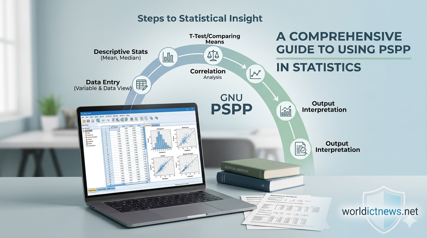
A Comprehensive, Step-by-Step Guide to Using PSPP in Statistical Analysis. Data analysis is a core pillar of modern research, business intelligence, and academic study. While proprietary tools like IBM SPSS Statistics dominate the landscape, its licensing fees present a significant financial barrier for students, independent researchers, and non-profit organizations.Fortunately, the GNU Project developed PSPP, a completely free, open-source alternative to SPSS. PSPP mirrors the user interface, syntax language, and data organization layout of SPSS, allowing users to transition seamlessly without a steep learning curve.This comprehensive, step-by-step article serves as a practical manual for executing statistical analyses in PSPP. We will cover environment setup, data entry, descriptive statistics, and hypothesis testing—complete with real-world sample questions, step-by-step navigation instructions, and data output interpretations.Understanding the PSPP EnvironmentWhen you open the PSPPire Graphical User Interface (GUI), you are presented with a primary workspace known as the Data Editor. Just like SPSS, this editor features two distinct views toggled at the bottom left-hand corner of the screen:Variable View: The design canvas where you define your variables, configure data types (e.g., numeric, string, date), adjust width, specify decimal places, and assign descriptive labels or value codes.Data View: A spreadsheet-like grid where the rows represent distinct observations (cases/participants) and the columns represent the variables defined in the Variable View.Statistical analysis results do not appear in the Data Editor. Instead, running any statistical command automatically triggers a separate pop-up window known as the Output Viewer, where tables, metrics, and text summaries are formatted for review.Section 1: Setting Up Variables and Entering DataBefore running any test, data must be structured correctly. Let us explore how to build a basic dataset from scratch using a hypothetical research scenario.ScenarioA researcher wants to study the relationship between a person’s biological sex, their age, and their performance on a standard cognitive memory test (scored from 0 to 100).Step-by-Step Dataset Construction1. Define Variables in Variable ViewClick the Variable View tab at the bottom left. Set up three distinct variables in successive rows:Variable 1: SexName: SexType: NumericDecimals: 0Label: Biological Sex of ParticipantValue Labels: Click the ellipsis (...) cell. Add 1 = Male and 2 = Female. This allows PSPP to process categorical data mathematically while displaying readable categories.Measure: NominalVariable 2: AgeName: AgeType: NumericDecimals: 0Label: Age in YearsMeasure: ScaleVariable 3: ScoreName: ScoreType: NumericDecimals: 2Label: Cognitive Test Performance ScoreMeasure: Scale2. Input Observations in Data ViewSwitch to the Data View tab. Enter the raw data points into rows like a conventional spreadsheet:Row (Case)SexAgeScore112185.50222492.00312278.00421988.50513565.00622995.00723189.00812672.50Section 2: Descriptive StatisticsDescriptive statistics summarize and describe the core characteristics of a dataset. They give analysts a bird's-eye view of central tendencies and data distributions.Question 1What are the mean, median, standard deviation, and range of the respondents’ ages and cognitive test scores in our sample?Step-by-Step PSPP ExecutionNavigate to the top menu bar and click AnalyzeDescriptive StatisticsFrequencies.A dialog box will appear. Select Age in Years [Age] and Cognitive Test Performance Score [Score] from the left variable list.Click the arrow button to move them into the Variable(s) column on the right.Click the Statistics button at the bottom of the dialog box.Check the boxes for Mean, Median, Std deviation, Minimum, and Maximum.Click Continue, and then click OK.Output InterpretationThe Output Viewer will generate a summary table resembling the following:MetricAge in YearsCognitive Test Performance ScoreN (Valid)88Mean25.8883.19Median25.0087.00Std. Deviation5.2510.37Minimum1965.00Maximum3595.00Analysis conclusion: The average age of our sample is 25.88 years (with a standard deviation of 5.25), ranging from 19 to 35. The average performance score sits at 83.19 points, showing a relatively tight spread (SD = 10.37) around a median performance of 87.00.Section 3: Comparing Means (Independent Samples t-Test)An independent samples t-test compares the mean scores of two unrelated groups to determine whether there is statistical evidence that the associated population means are significantly different.Question 2Is there a statistically significant difference in cognitive test scores between male and female participants?Step-by-Step PSPP ExecutionGo to the top menu and select AnalyzeCompare MeansIndependent-Samples T Test.Select Cognitive Test Performance Score [Score] and move it into the Test Variable(s) field.Select Biological Sex of Participant [Sex] and move it into the Grouping Variable field.Click Define Groups. Enter 1 for Group 1 (representing Males) and 2 for Group 2 (representing Females).Click Continue, then click OK.Output InterpretationThe output reveals two critical tables: Group Statistics and the Independent Samples Test.Group Statistics Table Summary:Male (N=4): Mean = 75.25; Std. Deviation = 9.35Female (N=4): Mean = 91.13; Std. Deviation = 2.95Independent Samples Test Table Summary:Levene's Test for Equality of Variances: Sig. (p-value) < 0.05 (Variances are unequal, meaning we must read the "Equal variances not assumed" row).t-value: -3.22df (Degrees of Freedom): 3.63Sig. (2-tailed): 0.038Analysis conclusion: Because the 2-tailed significance value (p = 0.038) is less than our standard alpha level of 0.05, we reject the null hypothesis. There is a statistically significant difference between groups: female participants scored significantly higher on the cognitive test than male participants.Section 4: Examining Relationships (Pearson Correlation)Correlation testing determines the strength and direction of a linear relationship between two continuous variables.Question 3Does an individual's age correlate significantly with their cognitive test score?Step-by-Step PSPP ExecutionGo to the top menu and click AnalyzeBivariate Correlation.Select both Age and Score from the left list.Click the arrow button to move them into the Variables box.Ensure the Pearson checkbox is marked under Correlation Coefficients.Keep Two-tailed significance selected.Click OK.Output InterpretationPSPP outputs a symmetrical correlation matrix table:VariableAgeScoreAgePearson CorrelationSig. (2-tailed)N1.008-0.8410.0098ScorePearson CorrelationSig. (2-tailed)N-0.8410.00981.008Analysis conclusion: The Pearson correlation coefficient () between Age and Score is -0.841. The significance value is 0.009, which is well below 0.05. This reveals a strong negative correlation that is statistically highly significant. As age increases, cognitive performance test scores tend to decrease significantly.Section 5: Categorical Data Analysis (Chi-Square Test of Independence)When both variables are nominal or ordinal (categorical), researchers use the Chi-Square test of independence to assess if the variables are associated with one another.Scenario ExpansionImagine expanding the sample to include a new categorical variable: Pass_Fail (1 = Pass, 2 = Fail). We want to know if passing rates differ across biological sexes.Question 4Is there a significant association between biological sex and the likelihood of passing or failing the cognitive evaluation?Step-by-Step PSPP ExecutionGo to the top menu and click AnalyzeDescriptive StatisticsCrosstabs.Move Sex into the Row(s) field.Move Pass_Fail into the Column(s) field.Click the Statistics button on the bottom right of the Crosstabs window.Check the box for Chi-square.Click Continue, and then click OK.Output InterpretationThe Output viewer produces a contingency table and a Chi-Square Tests diagnostic panel.Look closely at the Pearson Chi-Square row.Focus on the Asymp. Sig. (2-sided) column.Analysis conclusion: If the asymptotic significance value is greater than 0.05, you fail to reject the null hypothesis, concluding that biological sex is completely independent of pass/fail rates. Conversely, a value below 0.05 means sex is significantly associated with passing outcomes.Summary Comparison: PSPP vs. SPSSTo understand when to use PSPP over commercial choices, review this operational breakdown:Feature DimensionGNU PSPPIBM SPSS StatisticsLicensing CostCompletely Free (Open-Source)High Premium Commercial FeeInterface SetupDual-view layout (Variable & Data View)Dual-view layout (Variable & Data View)Core FunctionsFrequencies, T-Tests, ANOVA, Linear RegressionAdvanced Predictive Analysis, Neural NetworksPlatform SizeLightweight, runs efficiently on old hardwareHeavy download size, resource-demandingSyntax SupportInterprets SPSS command language directlyNative standard syntax language environmentConclusionPSPP is a powerful, lightweight, and accessible tool for anyone conducting statistical research without a massive software budget. By mastering variable definition, data entry, and core analytical paths—such as descriptives, independent t-tests, Pearson correlations, and cross-tabulations—you can answer complex research questions and extract deep insights from empirical data.

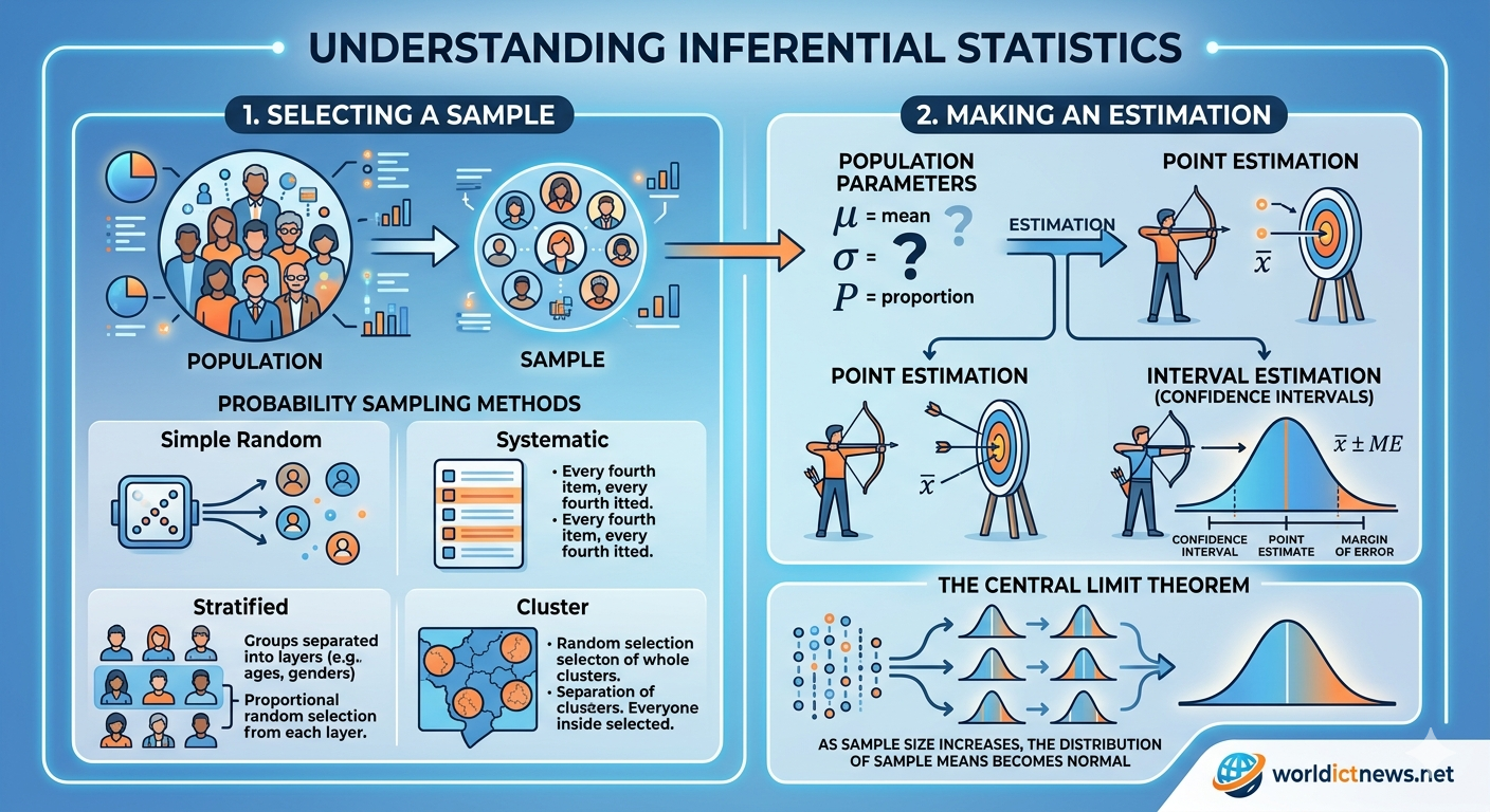
Mastering Inferential Statistics: A Comprehensive Guide to Sampling Methods and Estimation. Data is everywhere, but it is rarely practical to collect every piece of it. A multinational corporation cannot interview all eight billion people on Earth to test a new product. A medical research team cannot test a life-saving drug on every patient suffering from a specific disease.This logistical barrier is where inferential statistics becomes essential.Inferential statistics allows researchers to take a small, manageable portion of data and use it to make accurate predictions about a much larger group. This comprehensive guide explores the core framework of inferential statistics, focusing on two of its most critical pillars: sampling methods and estimation.1. The Core Framework: Population vs. SampleTo understand how inferential statistics works, you must first master the distinction between a population and a sample.Population: The entire group of individuals, objects, or measurements that you want to study. For example, all registered voters in a country, or every smartphone manufactured by a factory in a year.Sample: A smaller, representative subset selected from the larger population. For example, 1,500 voters selected for a polling survey.+------------------------------------------+| POPULATION || (Parameters: Mean μ, SD σ) || || +----------------------------+ || | SAMPLE | || | (Statistics: Mean x̄, s) | || +----------------------------+ |+------------------------------------------+Parameters vs. StatisticsData points change names depending on where they come from:Parameters: Numerical characteristics of a population (e.g., the true population mean, denoted by the Greek letter, or the population standard deviation, denoted by). These are usually unknown because measuring the entire population is impossible.Statistics: Numerical characteristics of a sample (e.g., the sample mean, denoted as, or the sample standard deviation, denoted as). These are calculated directly from your collected data.The core objective of inferential statistics is to use known sample statistics to estimate unknown population parameters.2. Sampling Methods: Building the FoundationThe validity of any statistical inference depends entirely on the quality of the sample. If a sample does not accurately reflect the diversity of the population, the resulting conclusions will be flawed. This flaw is known as sampling bias.Sampling methods are broadly divided into two categories: probability sampling and non-probability sampling.Probability Sampling MethodsIn probability sampling, every member of the population has a known, non-zero chance of being selected. This category is the gold standard for inferential statistics because it minimizes bias and allows for mathematical calculations of error.1. Simple Random Sampling (SRS)Every individual in the population has an equal chance of selection.How it works: Assign a number to every individual and use a random number generator to pick the sample.Example: Putting 100 employee names into a digital hat and drawing 10.Pros & Cons: Highly objective and easy to explain, but can be logistical nightmares for massive populations.2. Systematic SamplingMembers are selected at regular, predetermined intervals.How it works: Choose a random starting point, then select every-th individual from a ordered list (where).Example: Selecting every 20th car that rolls off an assembly line.Pros & Cons: Simpler and faster than SRS. However, if the population list has a hidden repeating pattern (periodicity), the sample will be highly biased.3. Stratified SamplingThe population is split into distinct, non-overlapping subgroups based on shared traits, called strata.How it works: Group the population by traits like age, gender, or income. Then, draw a random sample from each subgroup proportional to its size in the real population.Example: If a university is 60% undergraduate and 40% postgraduate, a stratified sample of 100 students will randomly pick exactly 60 undergraduates and 40 postgraduates.Pros & Cons: Ensures minority groups are fairly represented, increasing overall accuracy. The downside is that identifying and sorting individuals into clear strata requires deep prior knowledge of the population.4. Cluster SamplingThe population is divided into naturally occurring groups, called clusters, typically based on geography or organization.How it works: Instead of selecting individual people, you randomly select entire clusters and survey everyone inside those chosen clusters.Example: To study high school students in a state, randomly select 10 school districts (clusters) and interview every student in those 10 districts.Pros & Cons: Highly cost-effective and practical for large geographical areas. However, people within the same cluster often share similar views or traits, which can make the sample less representative than an SRS of the same size.Non-Probability Sampling MethodsIn non-probability sampling, elements are chosen based on convenience, judgment, or specific criteria, meaning not everyone has a chance to be selected. While easier and cheaper, these methods cannot be used to make rigorous statistical inferences because they introduce heavy bias.Convenience Sampling: Choosing individuals who are easiest to reach (e.g., interviewing people walking past you at a mall).Purposive (Judgmental) Sampling: The researcher uses their personal expertise to handpick a sample they believe fits the study's specific goals.Snowboard / Chain Sampling: Existing research participants recruit future participants from among their acquaintances (useful for hard-to-reach populations like underground subcultures).Quota Sampling: Setting a specific target number of people who meet certain criteria (e.g., "find 50 men and 50 women"), but filling those spots using convenience methods rather than random selection.3. The Central Limit Theorem (CLT): The Mathematical BridgeBefore moving from sampling to estimation, we must look at the mathematical engine driving inferential statistics: the Central Limit Theorem (CLT).Imagine taking a random sample of 30 people from a city, calculating their average height, and plotting it on a graph. Now imagine doing this 10,000 times. You would create a distribution of thousands of different sample means. This distribution is called the sampling distribution of the mean.The Central Limit Theorem states that:Normal Shape: If your sample size () is sufficiently large (usually), the sampling distribution of the mean will look like a bell-shaped curve (normal distribution). This remains true even if the underlying population distribution is completely skewed or irregular.Center: The average of all your sample means will exactly equal the true population mean ().Spread (Standard Error): The spread of these sample means is called the Standard Error (). It measures how much sample means fluctuate from sample to sample. It is calculated as:(Whereis the population standard deviation andis the sample size).The Central Limit Theorem is incredibly powerful. It proves that as your sample size grows larger, your sample mean becomes a highly reliable tracker of the true population mean.4. Estimation: Finding the True ValueOnce you have gathered a clean, random sample, you can use estimation to predict the true, hidden population parameters. Estimation is split into two strategies: Point Estimation and Interval Estimation.Point EstimationA point estimate uses a single calculated number from your sample to serve as the best guess for the population parameter.The sample mean () is the point estimate for the population mean ().The sample proportion () is the point estimate for the population proportion ().The Flaw of Point Estimates: While simple, point estimates are almost never 100% accurate. If your sample mean for employee satisfaction is 7.4 out of 10, it is highly unlikely the true population average is exactly 7.40000. It might be 7.3 or 7.5. A point estimate gives you a target, but it fails to communicate the margin of error or how confident you are in that number.Interval Estimation (Confidence Intervals)To fix the limitations of a point estimate, statisticians prefer Interval Estimation. This approach builds a range of plausible values around your point estimate, known as a Confidence Interval (CI).A confidence interval is structured as:Understanding the Confidence LevelA confidence interval is always tied to a confidence level (usually 95% or 99%).If you calculate a 95% Confidence Interval, it does not mean there is a 95% probability that the true population parameter sits inside that specific range. Instead, it means: "If we repeat this study with new random samples 100 times, 95 of the resulting intervals we calculate will successfully capture the true population parameter."Calculating a Confidence Interval for a Population Mean ()The exact formula depends on whether you know the true population standard deviation ().Scenario A: Whenis known (Using the Z-Distribution)(Whereis the critical value from the standard normal distribution based on your confidence level).For a 95% confidence level, the-value is 1.96.For a 99% confidence level, the-value is 2.58.Scenario B: Whenis unknown (Using the t-Distribution)In the real world, you almost never know the population standard deviation (). When it is missing, you must swap it out for your sample standard deviation () and use the Student's t-distribution instead of the standard Z-distribution.(Whererepresents degrees of freedom, calculated as).The-distribution looks similar to a normal distribution but has thicker tails. This shape accounts for the extra uncertainty that comes from estimating both the mean and the standard deviation at the same time. As your sample size () grows larger, the-distribution flattens out until it matches the standard-distribution.Visual Comparison of Distributions:Normal (Z) : _..---.._ (Thinner tails, higher peak)t-dist (df=5): .' _..._ '. (Thicker tails, handles uncertainty)5. Practical Example: Estimating Customer SpendingLet’s apply these theoretical steps to a practical business scenario.The ProblemAn e-commerce retailer wants to find the average amount of money spent per transaction on their website over the last year. They have millions of transactions, making it too slow and expensive to pull and clean the entire database. They decide to use inferential statistics.Step 1: SamplingThe retailer extracts an automated Simple Random Sample oftransactions from the past year. Because the sample size is greater than 30 (), the Central Limit Theorem applies, allowing them to proceed with confidence.Step 2: Calculate Sample StatisticsAfter running the numbers on the 100 sampled transactions, they find:Sample mean spending (): $85.00Sample standard deviation (): $20.00Step 3: Choose the Interval ModelBecause the true population standard deviation () is unknown, they must use the-distribution with degrees of freedom:Looking at a standard-table for a 95% confidence level with 99 degrees of freedom, the critical value is roughly:Step 4: Compute the Margin of Error (MoE)The margin of error is approximately $3.97.Step 5: Build and Interpret the IntervalConclusion: The retailer can state with 95% confidence that the true average spend across all millions of transactions falls somewhere between $81.03 and $88.97.Summary of Key Formulas and ConceptsConceptKey Formula / DefinitionPractical PurposeSimple Random SampleEqual chance selectionEliminates systemic biasCentral Limit TheoremProves large samples yield normal distributionsPoint EstimateorProvides a single, direct guess for a parameterConfidence Interval (Z)Used for interval estimation whenis knownConfidence Interval (t)Used for interval estimation whenis unknownConclusionInferential statistics changes data analysis from a passive backward glance into a forward-looking predictive tool. By understanding how to select an unbiased, random probability sample, you build a dependable foundation. By layering the Central Limit Theorem and interval estimation over that sample, you can extract deep insights about massive, complex populations using minimal data.Whether you are optimizing factory operations, tracking public opinion trends, or launching a new business project, mastering these foundational techniques protects you from relying on guesswork, letting you base your decisions on mathematically sound conclusions

Step-by-Step Probability Distribution Manual Calculation. In the fields of data science, machine learning, and statistical analysis, understanding how data points are distributed is foundational. While modern software pipelines and online calculators instantly compute statistical values, understanding the underlying mathematics is crucial for diagnosing modeling anomalies like data drift or skewed datasets.A Probability Distribution is a mathematical function that describes the likelihood of obtaining the possible values that a random variable can take. This comprehensive, hands-on guide walks you through the step-by-step manual calculation of a discrete probability distribution. You will learn how to build a manual probability distribution table, calculate the expected value (mean), compute the variance, and determine the standard deviation without relying on external software tools.1. Core Definitions: Random Variables and DistributionsTo build a probability distribution calculator manually, you must first understand the type of data you are processing. Random variables are divided into two primary categories:Discrete Random Variables: Variables that take on a countable number of distinct values (e.g., the number of servers failing in a data center, or the number of support tickets received per hour).Continuous Random Variables: Variables that take on an infinite number of possible values within a continuous range (e.g., the execution time of a cloud function, or network latency in milliseconds).This manual calculation guide focuses on Discrete Probability Distributions, which are governed by two mandatory mathematical axioms:The probability of each individual outcome x must sit between 0 and 1 inclusive:0 <= P(X = x) <= 1The sum of all individual probabilities across the entire sample space must equal exactly 1:Sum of P(x) = 12. Setting Up the Scenario Sample SpaceLet us establish a practical IT infrastructure scenario to serve as our calculation baseline.Suppose a DevOps engineering team tracks a cluster of 3 load balancers. Over a historical monitoring period, they record how many load balancers experience a localized configuration sync error during an automated deployment cycle.The sample space for the number of affected load balancers (x) ranges from 0 to 3. Based on log frequency data, the underlying probability values are recorded as follows:Probability of 0 errors: 0.40Probability of 1 error: 0.35Probability of 2 errors: 0.15Probability of 3 errors: 0.10Step 1: Verify the Distribution AxiomBefore executing advanced calculations, calculate the sum of your probabilities to verify the dataset is statistically valid:Sum of P(x) = 0.40 + 0.35 + 0.15 + 0.10 = 1.00The sum equals exactly 1.00, confirming the dataset is a valid probability distribution.3. Constructing the Calculation TableThe most effective tool for manual distribution calculation is a multi-column matrix table. This structural layout breaks down complex formulas into simple arithmetic steps, reducing calculation errors.Create a blank ledger containing five core columns:x: The individual random variable outcomes.P(x): The corresponding probability of each outcome.x * P(x): The product used to calculate the Expected Value.(x - Mean): The deviation of each outcome from the calculated mean.(x - Mean)^2 * P(x): The weighted squared deviation used to calculate Variance.Let's populate the primary inputs:Outcome (x)Probability (P(x))x * P(x)(x - Mean)(x - Mean)^2 * P(x)00.40nill nillnill10.35nillnillnill20.15nillnillnill30.10nillnillnill4. Step-by-Step Calculation of Expected Value (Mean)The Expected Value, mathematically denoted as E(X) or the symbol Mean, represents the long-term average outcome if the random event were repeated an infinite number of times.The formula for the expected value of a discrete distribution is:Mean = Sum of [x * P(x)]Step 2: Calculate the product for each rowRow 1 (x=0): 0 * 0.40 = 0.00Row 3 (x=1): 1 * 0.35 = 0.35Row 3 (x=2): 2 * 0.15 = 0.30Row 4 (x=3): 3 * 0.10 = 0.30Step 3: Sum the productsAdd the values together to find the expected value (Mean):Mean = 0.00 + 0.35 + 0.30 + 0.30 = 0.95Statistical Interpretation: If the engineering team runs thousands of deployments, they can expect an average of 0.95 errors per deployment cycle.5. Step-by-Step Calculation of VarianceThe Variance, denoted as Variance or Var(X), measures the dispersion of the distribution. It quantifies how far the individual outcomes spread out from the expected value (Mean = 0.95) we just calculated.The formula for calculating variance manually is:Variance = Sum of [(x - Mean)^2 * P(x)]Step 4: Calculate the deviation column (x - Mean)Subtract the mean (0.95) from each individual outcome (x):Row 1 (x=0): 0 - 0.95 = -0.95Row 2 (x=1): 1 - 0.95 = 0.05Row 3 (x=2): 2 - 0.95 = 1.05Row 4 (x=3): 3 - 0.95 = 2.05Step 5: Square the deviations and multiply by P(x)Square each deviation result to eliminate negative signs, then multiply that result by the row's corresponding probability:Row 1 (x=0): (-0.95)^2 0.40 = 0.9025 0.40 = 0.3610Row 2 (x=1): (0.05)^2 0.35 = 0.0025 0.35 = 0.000875Row 3 (x=2): (1.05)^2 0.15 = 1.1025 0.15 = 0.165375Row 4 (x=3): (2.05)^2 0.10 = 4.2025 0.10 = 0.42025Step 6: Sum the weighted squared deviationsAdd the values from the final column to find the total variance:Variance = 0.3610 + 0.000875 + 0.165375 + 0.42025 = 0.94756. Step-by-Step Calculation of Standard DeviationWhile variance is mathematically valuable, its units are squared (e.g., "0.9475 errors squared"), making it difficult to interpret alongside raw data. To return to our baseline unit of measurement, we calculate the Standard Deviation.The standard deviation is simply the positive square root of the variance:Standard Deviation = Square Root of (Variance)Step 7: Extract the square rootUsing a standard manual calculations block for the Square Root of 0.9475:Standard Deviation = Square Root of (0.9475) = 0.9734Final Analysis Profile: Our calculated system profile shows an expected error rate of 0.95 errors with a standard deviation of 0.9734 errors. This indicates a high level of variability relative to the mean, signaling that error rates fluctuate significantly between different deployment cycles.7. The Completed Reference Ledger TableBelow is the fully calculated distribution table. This serves as the reference blueprint for verifying manual arithmetic:Outcome (x)Probability (P(x))x * P(x)(x - Mean)(x - Mean)^2 * P(x)00.400.00-0.950.36100010.350.35+0.050.00087520.150.30+1.050.16537530.100.30+2.050.420250Sum1.00Mean = 0.95—Variance = 0.9475ConclusionBuilding a probability distribution calculator manually requires a methodical, step-by-step approach to processing outcomes, probabilities, and statistical averages. By validating the baseline axioms, constructing a ledger table, and processing expected values, variance, and standard deviation sequentially, you can calculate discrete distributions accurately without software dependencies. This core mathematical workflow forms the foundation for data modeling, risk profiling, and complex algorithmic processing across tech and data sectors.Frequently Asked Questions (FAQ)1. What happens if the sum of my P(x) column does not equal 1?If the sum of your probabilities does not equal exactly 1.0, your dataset is structurally invalid or incomplete. Double-check your initial log figures for math errors, or ensure that you have accounted for every possible outcome in your sample space.2. Can an individual deviation value (x - Mean) be negative?Yes, individual deviation values will be negative whenever an outcome (x) is smaller than the calculated distribution mean. However, these negative values disappear in the next step when you square the deviations.3. What is the alternative formula for calculating variance manually?An alternative formula for variance is the computational formula: Variance = Sum of [x^2 * P(x)] - Mean^2. This method skips the individual deviation column by summing the products of the squared outcomes and probabilities, then subtracting the squared mean at the very end.4. What does a standard deviation close to 0 indicate?A standard deviation close to 0 indicates that the random variable outcomes are tightly clustered around the expected value, signaling high predictability and low variance across cycles.5. Is this manual calculation method applicable to continuous variables?No, this specific tabular summation method applies only to discrete random variables. Continuous random variables require integral calculus over a specific probability density function (PDF) boundary to find mean and variance.

Understanding the Data Science Lifecycle: From Collection to Deployment. In the modern digital economy, data is frequently described as the new oil. However, raw data, much like unrefined petroleum, holds little inherent value. The true power of data lies in an organization's ability to extract actionable insights, build predictive systems, and automate decision-making processes. To transform chaotic datasets into strategic business assets, data professionals rely on a structured, iterative framework known as the Data Science Lifecycle.The Data Science Lifecycle serves as a roadmap for executing complex data projects. It ensures that data initiatives align with commercial objectives, maintain statistical integrity, and culminate in stable production deployments. Whether you are building an AI-powered product recommendation engine or analyzing customer churn trends, following this end-to-end lifecycle is critical to avoiding project failure. This comprehensive guide details the foundational phases of the lifecycle—from initial data acquisition to final model deployment.1. Business Understanding and Problem DefinitionEvery successful data science project begins not with code or algorithms, but with clear business objectives. Jumping directly into data collection without defining a specific problem is one of the leading causes of enterprise data project cancellation.During this initial phase, data scientists collaborate closely with domain experts, product managers, and executive stakeholders to answer fundamental questions:What specific business problem are we trying to solve? (e.g., Reducing fraudulent financial transactions).What are the project constraints, timelines, and budget limitations?How will the success of the project be measured?+-------------------------------------------------------------------+| PROJECT METRIC ALIGNMENT || || Business Goal: Reduce Customer Churn || │ || ▼ || Data Science Metric: Optimize ROC-AUC / F1-Score for Fraud Class|+-------------------------------------------------------------------+This phase bridges the gap between commercial terminology and statistical metrics. For instance, if the business goal is to "improve customer retention," the data science team must translate this into a measurable modeling target, such as "building a binary classification model to predict which users have a high probability of canceling their subscription within the next 30 days."2. Data Acquisition and CollectionOnce the objective is established, the next step is gathering the raw material: data. Depending on the project scope, data can originate from a variety of sources, both internal and external to the enterprise.Data collection strategies generally fall into three categories:Internal Relational DatabasesMost corporate data resides within structured transactional databases. Data engineers and data scientists use Structured Query Language (SQL) to extract historical customer records, sales transactions, and product inventories from systems like PostgreSQL, MySQL, or enterprise data warehouses like Snowflake and Google BigQuery.Application Log Files and Streaming DataFor real-time applications, data is continuously ingested via event streams. For example, tracking user clicks on an e-commerce website or gathering sensor metrics from IoT devices requires streaming pipelines managed by tools like Apache Kafka or AWS Kinesis.External APIs and Web ScrapingWhen internal data is insufficient, external datasets must be acquired. This involves programmatically pulling data via third-party Application Programming Interfaces (APIs), utilizing public datasets (such as those found on Kaggle or government repositories), or leveraging web scraping frameworks like Beautiful Soup and Scrapy to extract unstructured web text.3. Data Cleansing and PreprocessingRaw data is rarely clean. It is often riddled with missing values, duplicate entries, formatting inconsistencies, and statistical anomalies. Data cleansing—frequently called data wrangling—is the most time-consuming phase of the lifecycle, often consuming up to 70% to 80% of a data scientist's total workflow.Raw Data ──► [ Deduplication ] ──► [ Imputation ] ──► [ Type Casting ] ──► Clean DataKey preprocessing operations include:Handling Missing ValuesData records frequently contain blank entries. Data scientists must decide whether to remove rows with missing attributes entirely or fill them using statistical estimation techniques known as imputation (e.g., replacing a missing age value with the column's mean or median).Eliminating Duplicates and Corrupted RowsSystem glitches can cause duplicate records or corrupt entries. Identifying and purging these anomalies ensures that machine learning models are not trained on skewed or incorrect inputs.Data Type StandardizationsData must be correctly formatted before mathematical processing. This involves converting string characters into numerical values, standardizing datetime fields across uniform time zones, and ensuring categorical elements (like "True/False" or "Yes/No") are parsed systematically.4. Exploratory Data Analysis (EDA)With clean data in hand, data scientists perform Exploratory Data Analysis (EDA). The objective of EDA is to explore the dataset's underlying structure, identify patterns, detect anomalies, and test hypotheses using visual and statistical summaries. [ Histogram ] [ Scatter Plot ] [ Heatmap ] Distribution Check Correlation Detection Multicollinearity CheckEDA typically leverages three core visualization techniques:Histograms and Box Plots: Used to examine the distribution of individual variables and isolate extreme values (outliers) that could distort future predictions.Scatter Plots: Utilized to map two distinct variables against one another, revealing hidden linear or non-linear correlations.Correlation Heatmaps: Used to analyze the linear relationships across all numerical columns simultaneously. This helps identify multicollinearity, a condition where two input features are highly correlated, potentially degrading the stability of certain machine learning models.5. Feature Engineering and SelectionFeature engineering is the process of using domain knowledge to transform raw variables into more informative inputs (features) that enhance the predictive accuracy of machine learning models.Feature Transformation ExamplesTemporal Extractions: Extracting specific data components from a single timestamp field, such as converting "2026-05-16 18:35:00" into categorical components like "Day of Week: Saturday" or "Hour: 18".One-Hot Encoding: Converting text-based categorical variables (such as a "Country" column containing values like "USA", "UK", or "Nigeria") into separate binary columns containing 0s and 1s, which algorithms can process mathematically.Feature Scaling: Normalizing numerical variables to sit within a uniform scale (e.g., between 0 and 1) using techniques like Min-Max Scaling or Standardization. This prevents features with large numeric scales (like annual income) from over-indexing against smaller scales (like age).Feature SelectionIncluding too many variables can cause models to overfit, slow down training times, and increase computational costs. Feature selection algorithms help isolate the most important predictors while discarding redundant or irrelevant data columns.6. Model Training and ValidationThis phase is where predictive modeling takes place. Data scientists select appropriate machine learning algorithms based on the problem definition established in phase one.Entire Dataset ├── Train Set (80%) ──► Train Model Adjusting Weights └── Test Set (20%) ──► Evaluate Unseen GeneralizationAlgorithm CategoriesRegression Models: Used for predicting continuous numerical outputs (e.g., Linear Regression or Random Forest Regressors to predict housing prices).Classification Models: Used for predicting discrete categorical outputs (e.g., Logistic Regression, Support Vector Machines, or Gradient Boosting Classifiers to determine if an email is "Spam" or "Not Spam").Clustering Models: Unsupervised techniques used to group unlabelled data points based on geometric proximity (e.g., K-Means clustering for market segmentation).Training and Testing SplitTo ensure a model can generalize effectively to new data, the dataset is split into two parts: a Training Set (typically 80%) used to build the model, and a Testing Set (typically 20%) kept isolated. Evaluating the model against the testing set provides an unbiased assessment of its real-world performance.7. Model EvaluationBefore a model is allowed to influence business operations, its performance must be validated against standardized metrics. Relying solely on basic "Accuracy" can be highly misleading, especially when dealing with unbalanced datasets.Consider a fraud detection system where only 1% of transactions are actually fraudulent. A broken model that simply guesses "Not Fraud" for every transaction will technically achieve 99% accuracy, while failing completely at its actual objective. Data scientists rely on more robust evaluation metrics to measure true performance: ACTUAL VALUES True False PREDICTED +--------+-----------+ VALUES | TP | FP | --> Precision = TP / (TP + FP) +--------+-----------+ | FN | TN | --> Recall = TP / (TP + FN) +--------+-----------+Precision: Measures the proportion of predicted positive instances that were actually correct. This is critical when false positives are expensive.Recall (Sensitivity): Measures the proportion of actual positive instances that the model successfully caught. This is vital in scenarios like medical diagnostics or fraud detection, where missing a true positive has severe consequences.F1-Score: The harmonic mean of Precision and Recall, providing a balanced metric for uneven datasets.ROC-AUC Score: Evaluates how well a classification model separates different classes across various decision thresholds.8. Deployment and MLOpsThe final phase of the Data Science Lifecycle moves the trained model out of the local development environment (like Jupyter Notebooks) and into a production ecosystem where apps and end-users can access it in real time. This transition falls under the domain of MLOps (Machine Learning Operations).[ Local Notebook ] ──► [ Docker Container ] ──► [ REST API Endpoint ] ──► [ Web App ]A standard deployment workflow follows these operational steps:Containerization with DockerThe model files, code libraries, dependencies, and configuration settings are packaged together into a isolated Docker Container. This guarantees that the model runs identically regardless of whether it is hosted on a local testing laptop or an enterprise cloud cluster.Exposing as a REST APIThe containerized model is wrapped in a lightweight web framework like FastAPI or Flask and deployed as an active API endpoint. External applications can send data to this endpoint via JSON requests and receive live model predictions within milliseconds.Production InfrastructureAPI endpoints are scaled across cloud infrastructure using orchestration tools like Kubernetes, or serverless deployment pipelines like AWS SageMaker, Azure ML, or Google Vertex AI.Continuous Monitoring and Drift DetectionDeploying a model is not a one-time event. Over time, real-world data distributions change, causing a drop in predictive accuracy—a phenomenon known as Model Drift or Data Drift. Production monitoring pipelines track incoming data and trigger automated retraining loops when performance dips below acceptable thresholds.ConclusionThe Data Science Lifecycle is a structured, end-to-end framework that converts raw data into reliable, production-ready systems. Navigating from initial business alignment through cleansing, feature engineering, modeling, and MLOps deployment requires careful execution at every step. By adhering to this lifecycle, organizations can build robust analytics frameworks that add measurable, scalable value to their digital infrastructure.Frequently Asked Questions (FAQ)1. Why is Exploratory Data Analysis (EDA) important before machine learning?EDA helps data scientists understand the underlying patterns, structure, and quality of a dataset before training models. Skipping EDA can lead to training algorithms on skewed data, missing critical feature correlations, or failing to identify outliers that distort predictive accuracy.2. What is the difference between Precision and Recall?Precision measures the accuracy of positive predictions (out of all examples predicted as positive, how many were true). Recall measures the model's ability to find all positive instances (out of all actual positive examples, how many were correctly caught).3. What causes Model Drift in production environments?Model Drift occurs when the real-world data an active model encounters shifts away from the historical data it was originally trained on. Changes in consumer behavior, macroeconomic trends, or system updates can alter data patterns, making older predictions less accurate over time.4. What role does Docker play in the Data Science Lifecycle?Docker standardizes model deployment by packaging code, runtime environments, and dependencies into an isolated container. This eliminates the "it works on my machine" problem, ensuring the model functions consistently across local machines, staging areas, and live cloud environments.5. Why does data cleaning take up the majority of a project's timeline?Real-world data is routinely collected from uncoordinated logs, user inputs, and legacy databases. Resolving missing values, fixing corrupted formats, and standardizing datatypes requires meticulous programmatic checks to avoid feeding low-quality data into machine learning models.

How Advanced Data Analytics Prevents Financial Fraud in Modern Banking. The global banking ecosystem is undergoing an unprecedented digital transformation. As institutions shift from legacy physical branches to cloud-native mobile applications, instant payment rails, and decentralized financial architectures, the speed of commerce has accelerated exponentially. Today, billions of dollars cross international borders in milliseconds. However, this friction-less digital experience has introduced an equally sophisticated, hyper-connected threat matrix: automated, distributed financial fraud.Traditional, rules-based fraud detection systems—built on static, "if-then" logic structures—are no longer capable of keeping pace with modern criminal syndicates. These legacy tools are inherently reactive, flagging anomalies only after a vulnerability has been exploited. To shield institutional capital and maintain consumer trust, the financial sector must pivot toward proactive, predictive intelligence.Data analytics, driven by machine learning pipelines, real-time streaming architectures, and behavioral telemetry, has emerged as the foundational pillar of modern banking defense. By processing petabytes of transactional, behavioral, and contextual data simultaneously, financial institutions can identify, isolate, and neutralize fraudulent activities in mid-air before a single cent leaves the network.1. The Anatomy of Modern Financial FraudTo appreciate the disruptive impact of data analytics, one must first analyze the highly technical nature of modern banking fraud. Cybercriminals leverage automated infrastructure, residential proxy networks, and generative artificial intelligence to mimic legitimate consumer profiles.Synthetic Identity TheftSynthetic identity fraud is one of the fastest-growing financial crimes globally. Instead of stealing a real person's complete identity, malicious actors harvest fragments of real credit data (such as stolen Social Security Numbers or national identity tokens) and combine them with completely fabricated personal details (false names, synthetic addresses, and newly registered burner phone numbers). Over several months, these synthetic profiles apply for minor lines of credit, build positive repayment histories, and suddenly "spin out"—maxing out major institutional loans and vanishing without a trace.Account Takeover (ATO) AttacksAccount Takeovers occur when unauthorized entities gain complete administrative control of a legitimate customer’s banking profile. These breaches are rarely executed via simple manual password guessing. Instead, malicious actors deploy automated credential-stuffing botnets across cloud infrastructure, testing millions of leaked username and password combinations across banking login portals within minutes. Once inside, they rapidly alter contact phone numbers, disable multi-factor authentication (MFA) parameters, and drain liquid assets via untraceable peer-to-peer wire transfers.Authorized Push Payment (APP) ScamsUnlike direct hacks, APP scams exploit human psychology. Attackers use sophisticated social engineering, business email compromise (BEC) frameworks, or deepfake audio to convince legitimate users, business accountants, or corporate treasurers to willingly authorize high-value wire transfers to shell corporate accounts. Because the actual transaction is initiated by an authorized user using their correct security tokens, legacy fraud systems see the payment as entirely legitimate.2. The Core Analytics Framework: Transitioning from Rules to PredictionLegacy banking applications protect accounts using static rulesets, such as: "If a transaction exceeds $10,000 and occurs outside the home country, flag for manual review."While straightforward, this approach exhibits two catastrophic flaws:Massive False Positive Rates: Legitimate travelers making normal purchases are locked out of their accounts, destroying the user experience.Susceptibility to Reverse Engineering: Professional fraudsters rapidly test transaction amounts (e.g., executing charges of $9,995 instead of $10,000) to map out and bypass a bank's defensive limits.Advanced data analytics solves this by replacing binary rules with multi-dimensional, continuous risk scoring.[ Incoming Transaction ] │ ├──> Behavioral Telemetry Analytics ───┐ ├──> Graph Theory Network Mapping ──────┼─> [ Machine Learning Engine ] ─> [ Continuous Risk Score ] └──> Device Fingerprint Analytics ─────┘ │ ├──> Score < 30 : Approve Automatically ├──> Score 30-70 : Trigger Adaptive MFA └──> Score > 70 : Instant Freeze & Decline3. Key Analytic Techniques Driving Fraud PreventionTo build a comprehensive, multi-layered fraud prevention stack, banks run three primary data analytics workflows simultaneously across their core processing engines.1. Behavioral Biometrics and User TelemetryEvery human interacts with digital devices in a highly distinct, idiosyncratic manner. Behavioral analytics models ingest unstructured telemetry data directly from mobile apps and web frontends to build an invisible, continuous biometric profile for each client.Keystroke Dynamics: Analyzing the exact millisecond dwell time (how long a key is held down) and flight time (the gap between keys) during a login attempt.Touchscreen Pressures & Angles: Measuring how firmly a user presses their smartphone screen and the precise angle at which they hold the device.Mouse Trajectory Vectoring: Track real-time cursor paths. Real humans move mice in erratic, curved vectors with natural micro-pauses; automated botnets move in perfect, computationally optimal straight lines.If an account logs in with the correct password and passes MFA, but the typing speed and finger pressure vectors match a known botnet signature or a distinct profile, the system instantly triggers an out-of-band identity verification step.2. Graph Database Analytics and Network TopologyFraudsters rarely operate in complete isolation; they rely on interconnected webs of mule accounts, shell companies, and shared digital infrastructure to launder stolen funds. Traditional relational databases (SQL) struggle to track these relationships because mapping deep links across billions of columns requires complex, computationally expensive table joins.Graph analytics utilizes specialized graph databases (such as Neo4j or Amazon Neptune) to treat data as nodes (entities like accounts, names, or devices) and edges (the relationships between them).[ Stolen Device ID ] ──(Shared Link)──> [ Fraudulent Account A ] │ (Rapid Transfer) ▼ [ Mule Account B ] │ (Rapid Transfer) ▼ [ Shell Company C ]By visualizing the banking network as an interconnected topology, graph analytics can detect Fraud Rings instantly. If the system observes ten separate bank accounts opened by completely different individuals, but notes that all ten profiles share a single, hidden variable—such as a matching hardware MAC address or an identical employer tax ID—the graph network flags the entire cluster as a synthetic identity setup before a single credit line can be drawn.3. Real-Time Streaming Analytics and Event ProcessingFraud occurs at machine speed; therefore, remediation must occur at machine speed. Modern banking architectures utilize streaming data platforms like Apache Kafka or Amazon Kinesis to intercept transaction payloads in transit.As a payment request is initiated, the streaming engine matches the event against historical baseline data within a tight 200-millisecond window. The model runs predictive algorithms evaluating historical location drift, spending velocities, merchant categorization codes, and device health. If the transaction deviates significantly from the user's localized spatial-temporal habits, the pipeline changes the transaction state to "Pending Verification," freezing the assets safely before the outbound wire clears the clearinghouse.4. The Engineering Blueprint: Implementing AI/ML Fraud PipelinesBuilding an enterprise-grade analytics engine requires an integrated data engineering pipeline that can handle both massive batch training and ultra-fast real-time scoring.Architecture TierTechnological ToolingPrimary Operational RoleData IngestionApache Kafka, AWS KinesisCaptures clickstream logs, device telemetry, and raw financial transactions concurrently.Storage & Feature StoreSnowflake, Databricks, FeastHouses historical raw logs and processes calculated features (e.g., 24-hour rolling transfer velocity).Model Processing EngineApache Spark, PyTorch, XGBoostExecutes complex machine learning inferences and predictive classification modeling within milliseconds.Orchestration LayerApache Airflow, KubeflowAutomates the continuous retraining, validation, and deployment of updated ML models.Feature Engineering: The Secret to High AccuracyThe predictive accuracy of any AI model rests entirely on the quality of its features. In a financial context, feature engineering takes raw transaction points and translates them into meaningful metrics. For example, instead of passing a raw transaction amount ($500) to an algorithm, data scientists engineer dynamic variables such as:ratio_ of _current_ amount_ to_ historical_ average _30dvelocity _of_ transactions_ in_ last _60_ minutesdistance_ between_ physical_ merchant_ and_ last_ atm_ withdrawalBy providing the machine learning model with highly descriptive, contextual variables, the algorithm can accurately separate an unusual but completely legitimate holiday shopping spree from an actual, active account draining operation.5. Overcoming Ethical and Operational ObstaclesWhile data analytics offers immense power, banking institutions must navigate critical regulatory, privacy, and infrastructure challenges when deploying these systems at scale.Managing False PositivesLocking an active card or freezing a business payroll account due to an incorrect fraud algorithm causes immense customer frustration and reputational damage. Banks must implement Explainable AI (XAI) frameworks. If a model flags a transaction as fraudulent, it cannot simply output a black-box answer. It must provide clear, auditable reasons (e.g., "Flagged due to a 400% deviation in typical transaction value combined with an unverified browser footprint"). This allows customer support teams to resolve issues transparently and efficiently.Regulatory Compliance and Data PrivacyFinancial analytics operates under strict global compliance mandates, including the General Data Protection Regulation (GDPR), Payment Card Industry Data Security Standard (PCI-DSS), and Know Your Customer (KYC) mandates. Banks cannot blindly store unencrypted consumer data in public cloud environments for analytics modeling. Data engineering teams must implement advanced anonymization, tokenization, and differential privacy methodologies, ensuring that models learn transactional patterns without ever exposing the sensitive, personally identifiable information (PII) of individual consumers.Conclusion: The Future of Autonomous Financial DefenseData analytics has completely shifted the power dynamics of global risk management. Financial fraud is no longer an unavoidable operational cost of doing business online; it is an engineered problem that can be actively managed, contained, and neutralized through continuous data intelligence.As cybercriminals continue to integrate sophisticated artificial intelligence into their offensive arsenals, the banking sector's defensive architectures must evolve in parallel. The institutions that thrive in this digital-first era will be those that view data analytics not merely as an IT support tool, but as a core, strategic shield—an autonomous, self-learning ecosystem capable of protecting global capital, preserving system integrity, and maintaining human trust at machine speed.

Probability Distribution - Function, Formula, Table. A probability distribution is a mathematical function that assigns the probabilities of different outcomes to the possible values of a random variable. It provides a way of modeling the likelihood of each outcome in a random experiment.While a Frequency Distribution shows how often outcomes occur in a sample or dataset, a probability distribution assigns probabilities to outcomes abstractly, theoretically, regardless of any specific dataset. These probabilities represent the likelihood of each outcome occurring. Common types of probability distributions include:Probability DistributionProperties of a probability distribution include:The probability of each outcome is greater than or equal to zero.The sum of the probabilities of all possible outcomes equals 1.In this article, we will cover the key concepts of probability distribution, types of probability distribution, along with the applications in CS.Probability Distribution of a Random VariableNow the question comes, how to describe the behavior of a random variable?Suppose that our Random Variable only takes finite values, like x1, x2, x3,... and xn. i.e., the range of X is the set of n values is {x1, x2, x3,... and xn}.The behavior of X is completely described by giving probabilities for all the values of the random variable X.EventProbabilityx1P(X = x1)x2P(X = x2)x3P(X = x3)The Probability Function of a discrete random variable X is the function p(x) satisfying.P(x) = P(X = x)Random VariableExample: We draw two cards successively with replacement from a well-shuffled deck of 52 cards. Find the probability distribution of finding aces.Answer: Let's define a random variable "X", which means number of aces. Since we are drawing two cards with replacement from a deck of 52 cards , X can only take on the values 0,1 or 2 as the cards are drawn with replacement, the two draws are independent experiments.Calculating the probabilities:P(X = 0) = P(both cards are non-aces)= P(non-ace) x P(non-ace) = 4852×4852=1441695248​×5248​=169144​P(X = 1) = P(one of the cards in ace) = P(non-ace and then ace) + P(ace and then non-ace)= P(non-ace) x P(ace) + P(ace) x P(non-ace)= 4852×452 +452×4852=241695248​×524​ +524​×5248​=16924​P(X = 2) = P(Both the cards are aces) = P(ace) x P(ace)= 452×452=1169524​×524​=1691​Now we have the probability distribution for the discrete random variable X. It can be represented in the following table:X 012P(X = x)144/16924/1691/169It should be noted here that each value of P(X = x) is greater than zero and the sum of all P(X = x) is equal to 1.Types of Probability DistributionsWe have seen what Probability Distributions are; now we will see different types of Probability Distributions. The Probability Distribution's type is determined by the type of random variable. There are two types of Probability Distributions:Discrete Probability Distributions for Discrete VariablesContinuous Probability Distribution for Continuous VariablesWe will study in detail two types of discrete probability distributions..Discrete Probability DistributionsDiscrete Probability Functions applies to discrete random variables, which take countable values (e.g., 0, 1, 2, …). These distributions assign probabilities to individual outcomes.It includes distributions such as Bernoulli, Binomial and Poisson, which are used to model outcomes that can be counted, as explained below:Bernoulli TrialsTrials of the random experiment are known as Bernoulli Trials, if they are satisfying below given conditions :Finite number of trials are required.All trials must be independent. (when the outcome of any trial is independent of the outcome of any other trial.) Every trial has two outcomes : success or failure.Probability of success remains constant across all trials.Example: Can throwing a fair die 50 times be considered an example of 50 Bernoulli trials if we define:Success is getting an even number (2, 4 or 6),Failure as getting an odd number (1, 3 or 5)Answer:Yes, this can be considered as example of 50 Bernoulli trailsThere are 3 even numbers out of 6 possible outcomes, so p = 3/6 = 1 /2There are 3 odd numbers out of 6, so q = 3/6 = 1 /2So, throwing a fair die 50 times with this definition is a classic example of 50 Bernoulli trials, with p=1/2 and q = 1/2Binomial DistributionThe binomial distribution models the number of successes (x) in n independent Bernoulli trials, each with success probability p.For example,For 1 success in 6 trials, there are 6 possible sequences (e.g., PQQQQQ, QPQQQQ, …PQQQQQ, QPQQQQ,…), each with probability p . (1−p)5Therefore the total Probability is given as = 6. p .(1-p)5Generalizing the idea, if Y is a Binomial Random Variable, the Probability Function P(Y) for the Binomial Distribution for n number of trials is given as:P(Y) = nCx px(1-p)n-x wherep is the probability of success in a given trial,'x' be the number of successes, x = 0,1,2...nExample: When a fair coin is tossed 10 times, find the probability of getting i. exactly six heads. ii. at least six heads.Answer:Every coin tossed can be considered as the Bernoulli trial. Suppose X is the number of heads in this experiment: We already know, n = 10, p = 1/2P(X = x) = nCx px(1-p)n-x  When x = 6, (i) P(x = 6) = 10C6 p6 (1-p) 4 = 10!6!4!(12)6(12)4 = 7×8×9×101×2×3×4×1210 = 2101024 = 1055126!4!10!​(21​)6(21​)4 = 1×2×3×47×8×9×10​×2101​ = 1024210​ = 512105​(ii) P(at least 6 heads) = P(X >= 6) = P(X = 6) + P(X=7) + P(X=8)+ P(X=9) + P(X=10) =10!6!4!(12)10+10!7!3!(12)10+10!8!2!(12)10+10!9!1!(12)10+10!10!(12)10 = (10!6!4!+10!7!3!+10!8!2!+10!9!1!+10!10!)(12)10 = (210+120+45+10+1)×11024=3861024 = 1935126!4!10!​(21​)10+7!3!10!​(21​)10+8!2!10!​(21​)10+9!1!10!​(21​)10+10!10!​(21​)10 = (6!4!10!​+7!3!10!​+8!2!10!​+9!1!10!​+10!10!​)(21​)10 = (210+120+45+10+1)×10241 ​= 1024386​ = 512193​Negative Binomial DistributionNegative binomial distribution models the number of trials (n) needed to get k successes, where successes are fixed, but trials vary.P(X=n)=n−1k−1pk(1−p)n−kP(X=n)=k−1n−1​pk(1−p)n−kWhere:n = total trials (including the k-th success),k = required successes (fixed),p = probability of success on a single trial,n−1k−1k−1n−1​ , the number of ways to arrange (k−1) successes in the first (n−1) trials.For example,Probability of getting exactly 3 coupons in 10 pizzas given that probability of success (per pizza): p=0.3k=3, p = 0.3, n = 10Therfore, total probability is P(X=10)=(29)(0.3)3(0.7)7≈0.08P(X=10)=(92​)(0.3)3(0.7)7≈0.08(8%)Poisson Probability DistributionThe Poisson distribution models the number of times an event occurs in a fixed interval of time or space. It is expressed asf(x; λ) = P(X = x) = (λxe-λ)/x!where,x is the number of times the event occurrede = 2.718...λ is the mean valueExample: A bakery sells an average of 5 cupcakes per hour. What’s the probability they sell exactly 3 cupcakes in the next hour?λ=5 (average rate), k=3 (desired events).P(X=x)=e−λλkx!P(X=3)=e−5533!≈0.14P(X=x)=x!e−λλk​P(X=3)=3!e−553​≈0.14Continuous Probability DistributionsProbability distributions for continuous random variables (uncountable outcomes, e.g., time, height, temperature), such as Uniform and Normal distributions, are explained below.Uniform DistributionUniform Distribution models equally likely outcomes over a closed interval [a,b], where the probability is uniform.Probability Density Function (PDF) of a Uniform Distribution is given by,f(x)={1b−aif a≤x≤b,0otherwise.f(x)={b−a1​0​if a≤x≤b,otherwise.​Cumulative Distribution Function (CDF) of a Uniform Distribution is given by,F(x)={0for x<a,x−ab−afor x∈[a,b],1for x>b.F(x)=⎩⎨⎧​0b−ax−a​1​for x<a,for x∈[a,b],for x>b.​Mean (μ): μ=a+b2μ=2a+b​​Variance (σ²): σ2=(b−a)212σ2=12(b−a)2​Example:Random number generator between 0 and 1.Normal (Gaussian) DistributionNormal distribution models symmetric, bell-shaped data around a mean (μ) with a spread (σ). It describes data that clusters around a central value, with probabilities decreasing exponentially as values deviate from the mean.PDF of Normal Distribution is given by,f(x)=1σ2πe−(x−μ)22σ2f(x)=σ2π​1​e−2σ2(x−μ)2​CDF of Normal Distribution is given by,F(x)=12[1+erf(x−μσ2)]F(x)=21​[1+erf(σ2​x−μ​)]Mean = Median = Mode = μ Variance = σ²Example:Heights of adults in a population (μ=170, σ=10).Chi-Square DistributionThe chi-square distribution used in hypothesis testing, especially for goodness-of-fit and independence tests. It only takes non-negative values and is positively skewed.Degrees of freedom refer to the number of independent values or quantities that can vary in the calculation of a statistic.For simple experiments, k = Number of Categories - 1In contingency table, k = (Rows - 1) × (Columns - 1)Mean: k Variance :2k, where k is the degree of freedomCritical values are used in hypothesis testing to determine whether observed frequencies in a contingency table differ significantly from expected frequencies.Example,Observed data; Oi: 55 heads, 45 tails in 100 flips.Expected (fair coin): Ei: 50 heads, 50 tails.Null Hypothesis (H0): The coin is fair (P(Heads)=0.5).Alternative Hypothesis (Ha​): The coin is biased.Chi-Square Statistic: χ2=∑(Oi−Ei)2Ei=(55−50)250+(45−50)250=1.0χ2=∑Ei​(Oi​−Ei​)2​=50(55−50)2​+50(45−50)2​=1.0Degrees of freedom: k = 2 − 1 = 1.  (since there are 2 categories: heads/tails).Critical value (α=0.05): χ0.952(1)=3.84χ0.952​(1)=3.84Since 1.0 < 3.84, fail to reject H0 (coin may be fair). The data does not show significant evidence of bias.Application of Probability Distribution in Computer ScienceProbability distributions are used in many areas of computer science are as follows:In machine learning, they help make predictions and deal with uncertainty.In natural language processing, they are used to model how often words appear.In computer vision, they help understand image data and remove noise.In networking, distributions like Poisson are used to study how data packets arrive.Cryptography uses random numbers based on probability.Software testing and reliability also use distributions to predict bugs and failures.Overall, probability distributions help in building smarter, more reliable and efficient computer systems.Solved Questions on Probability DistributionQuestion 1: A box contains 4 blue balls and 3 green balls. Find the probability distribution of the number of green balls in a random draw of 3 balls.Solution:Given that the total number of balls is 7 out of which 3 have to be drawn at random. On drawing 3 balls the possibilities are all 3 are green, only 2 is green, only 1 is green and no green. Hence X = 0, 1, 2, 3.P(No ball is green) = P(X = 0) = 4C3/7C3 = 4/35P(1 ball is green) = P(X = 1) = 3C1 × 4C2 / 7C3 = 18/35P(2 balls are green) = P(X = 2) = 3C2 × 4C1 / 7C3 = 12/35P(All 3 balls are green) = P(X = 3) = 3C3 / 7C3 = 1/35Hence, the probability distribution for this problem is given as followsX0123P(X)4/3518/3512/351/35Question 2: From a lot of 10 bulbs containing 3 defective ones, 4 bulbs are drawn at random. If X is a random variable that denotes the number of defective bulbs. Find the probability distribution of X.Solution:Since, X denotes the number of defective bulbs and there is a maximum of 3 defective bulbs, hence X can take values 0, 1, 2 and 3. Since 4 bulbs are drawn at random, the possible combination of drawing 4 bulbs is given by 10C4.P(Getting No defective bulb) = P(X = 0) = 7C4 / 10C4 = 1/6P(Getting 1 Defective Bulb) = P(X = 1) = 3C1 × 7C3/10C4 = 1/2P(Getting 2 defective Bulb) = P(X = 2) = 3C2 × 7C2/10C4 = 3/10P(Getting 3 Defective Bulb) = P(X = 3) = 3C3 × 7C1/10C4 = 1/30Hence Probability Distribution Table is given as followsX0123P(X)1/61/23/101/30Practice Problem Based on Probability Distribution FunctionQuestion 1. A coin is flipped 8 times. What is the probability of getting exactly 5 heads? (Assume the coin is fair.)Question 2. A dice is rolled until a 4 is rolled. If the first success (rolling a 4) occurs on the 6th roll, how many failures occurred before the success?Question 3. A customer service center receives an average of 3 calls per hour. What is the probability that they receive exactly 5 calls in an hour?Question 4. The heights of adult women in a certain population follow a normal distribution with a mean of 64 inches and a standard deviation of 3 inches. What is the probability that a randomly selected woman has a height greater than 66 inches?Question 5. For a continuous uniform distribution between 2 and 8, find the probability that the random variable is between 4 and 6.Question 6. A researcher performs a chi-square test to examine if there is a relationship between gender and voting preference in a survey of 150 people. The degrees of freedom for this test are 3. What is the critical value for the chi-square statistic at a 0.05 significance level?Question 7. A sample of 12 students was taken from a population to test their exam scores. The sample mean is 78 and the sample standard deviation is 5. Test if the sample mean significantly differs from a population mean of 75 at a 0.05 significance level.Question 8. In a factory, 95% of the machines work well and 5% are defective. If a machine is randomly selected and found to be defective, what is the probability that it was not properly maintained, given that 20% of the machines are poorly maintained? Use Bayes' Theorem to calculate this.Answer:-0.21875.50.1009.0.2546.0.3333.7.81.There is no significant difference between the sample mean and the population mean at the 0.05 significance level.11.11%.